Now, the actual measurement of my dipole with an ATU tuned at 7038kHz.
I get such values as:
...
7.037000 45.16 0.30
7.037500 45.31 0.19
7.038000 45.33 0.09
7.038500 45.29 -0.14
7.039000 45.28 -0.24
7.039500 45.44 -0.30
7.040000 45.31 -0.56
...
Let’s draw some graphs with gnuplot.
% gnuplot
gnuplot> plot "ant2.csv" using 1:2 with line linewidth 3, \
          "ant2.csv" using 1:3 with line linewidth 3
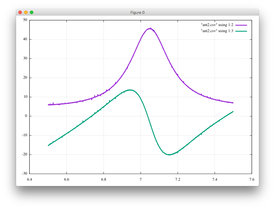
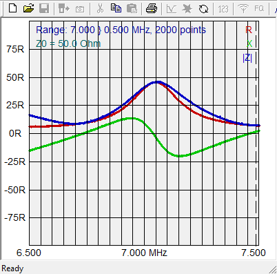
The frequency range is from 6.5MHz to 7.5MHz, and the purple line shows R [ohm], and the green line X [ohm], respectively.
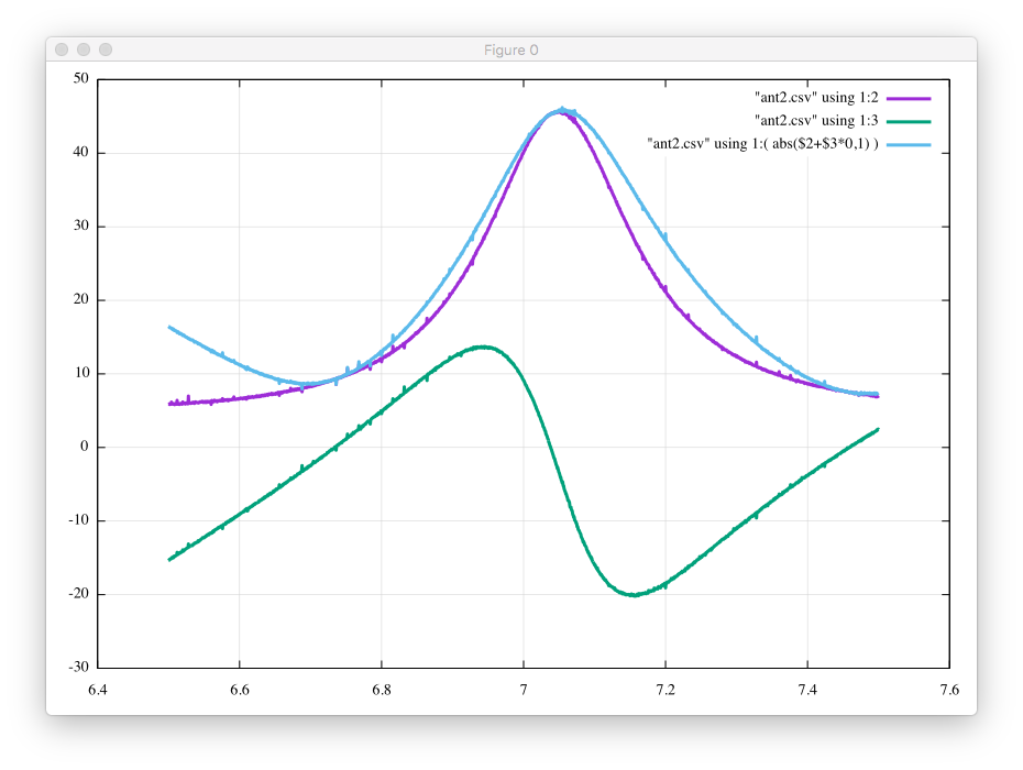
If you also want to show |Z|, the command is:
gnuplot> plot "ant2.csv" using 1:2 with line linewidth 3, \
          "ant2.csv" using 1:3 with line linewidth 3, \
          "ant2.csv" using 1:( abs($2+$3*{0,1}) ) with line linewidth 3
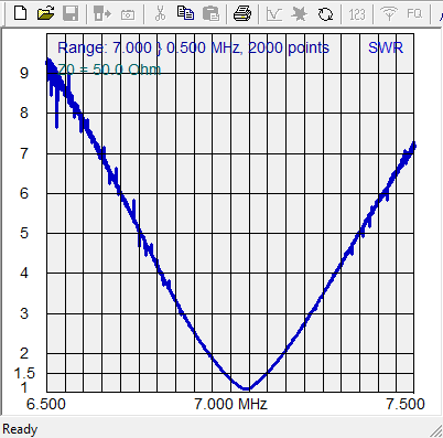
Using AntScope will give you the same kind of graph, but I believe you prefer to do it by yourself.
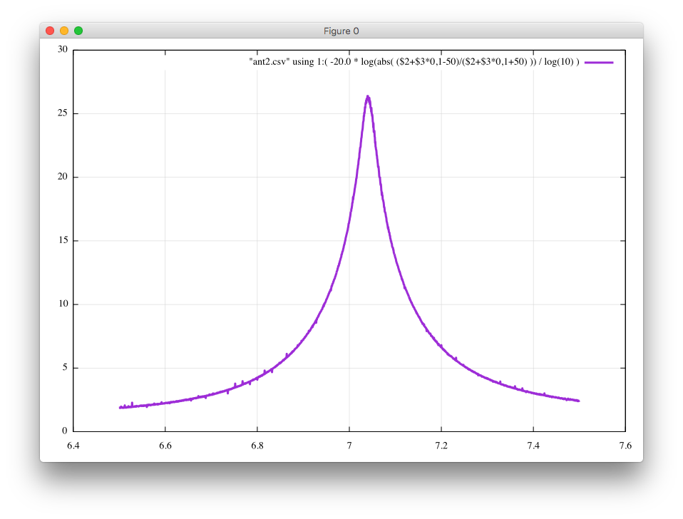
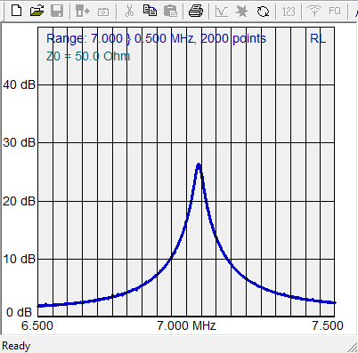
Return loss is obtained as follows:
gnuplot> plot "ant2.csv" using 1:( -20.0 * log(abs( ($2+$3*{0,1}-50)/($2+$3*{0,1}+50) )) / log(10) ) with line linewidth 3
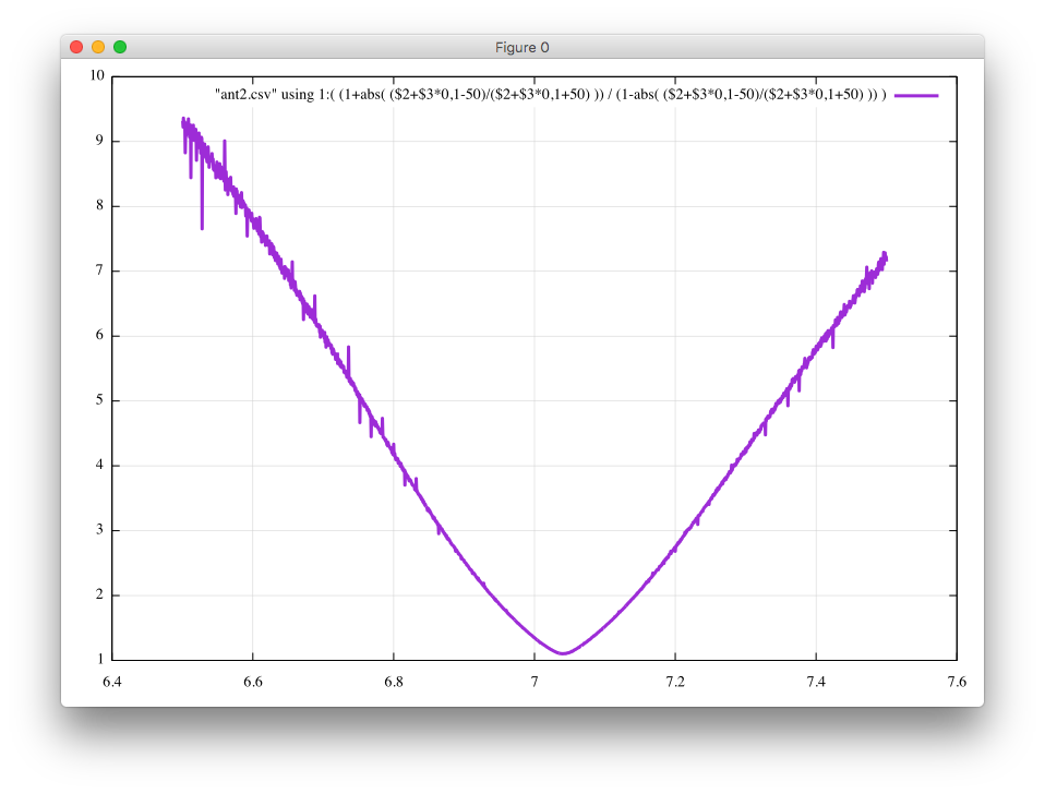
Finally, VSWR is:
gnuplot> plot "ant2.csv" using 1:( (1+abs( ($2+$3*{0,1}-50)/($2+$3*{0,1}+50) )) / (1-abs( ($2+$3*{0,1}-50)/($2+$3*{0,1}+50) )) ) with line linewidth 3