
My old site, http://spinor6.info/, will disappear on Sept. 28, 2013.
Dipole Antenna (5)
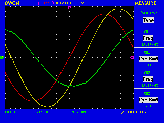
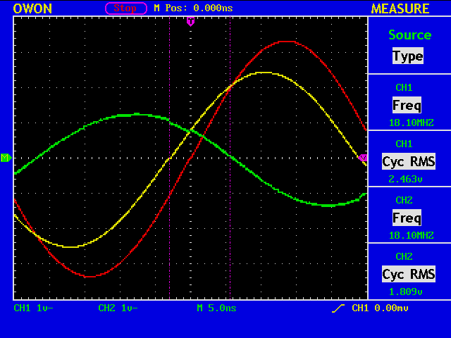
> Using the same elements and a cable, a 18MHz dipole is moved slightly in its position.
Moved again for a couple of feet or so.
gnuplot> load "gnuplot1.txt";
Freq [MHz]=18.1
V1=2.511
V2=2.751
Cursor 1=-5.6e-009
Cursor 2=-1.5e-008

vratio=1.09557945041816
phase1 [deg]=-36.4896
phase2 [deg]=-97.74

abs(gamma)=0.66232897357976
swr=4.92292451384606
cz={16.7351989530969, -38.8485688397987}
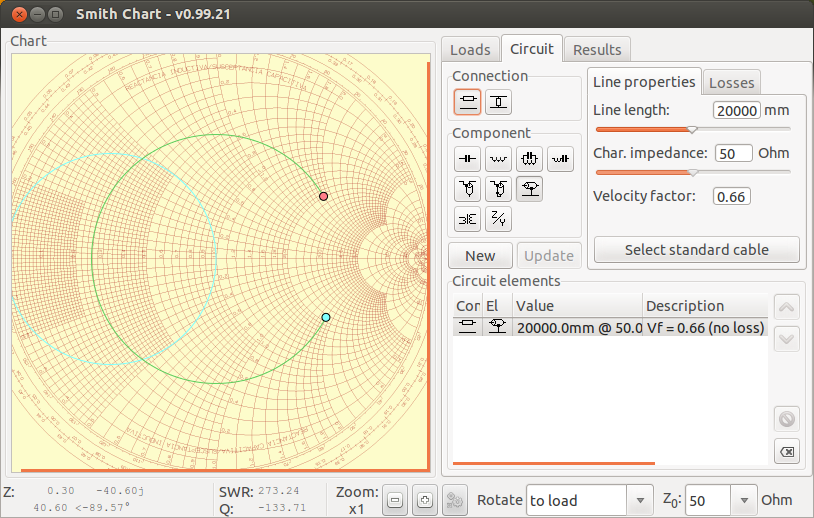
The impedance was previously cz={13.4238815578089, -32.7726324246538}, when the antenna was in its old position.
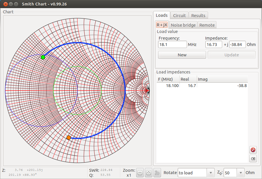
The new measured impedance of cz={16.7351989530969, -38.8485688397987} gives, considering the coax cable lenght of 20m, Zant={11.73, +19.24}, which happens to be almost on the g=1 circle.
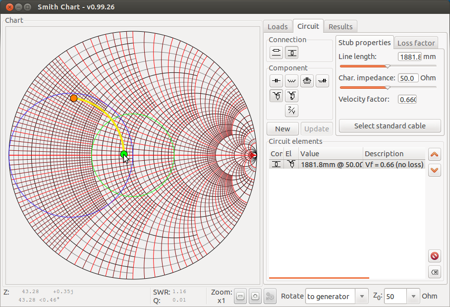
Therefore, an open stub of length 1881mm at the antenna feed point shall give you Z=43.28 ohm and SWR=1.16.
With a stub of length 2000mm, the following results are obtained.
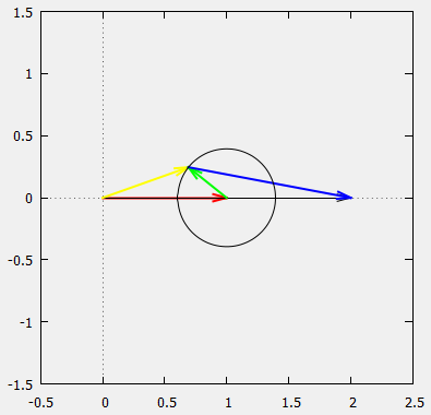
gnuplot> load "gnuplot1.txt"
Freq [MHz]=18.1
V1=2.463
V2=1.809
Cursor 1=3e-009
Cursor 2=-5.6e-009

vratio=0.734470158343484
phase1 [deg]=19.548
phase2 [deg]=-36.4896

abs(gamma)=0.393920800623182
swr=2.29989876249909
cz={23.8530134489064, 13.8771809482584}
The impedance of cz={23.8530134489064, 13.8771809482584} gives, Zant={37.947, -35.339}.
With a stub of length 1900mm, the following results are obtained.
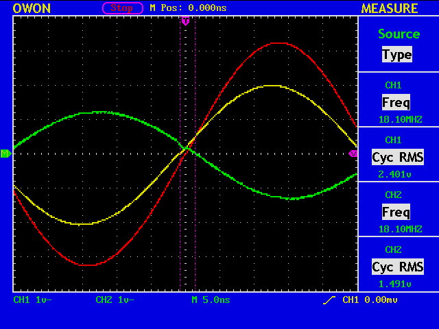
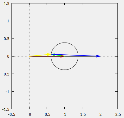
gnuplot> load "gnuplot1.txt"
Freq [MHz]=18.1
V1=2.401
V2=1.491
Cursor 1=8e-010
Cursor 2=-1.4e-009

vratio=0.620991253644315
phase1 [deg]=5.2128
phase2 [deg]=-9.1224

abs(gamma)=0.385725696138712
swr=2.25587443171256
cz={22.2605406131682, 2.9509421122626}
The impedance of cz={22.2605406131682, 2.9509421122626} gives, Zant={67.328, +45.316}.
At 18.1MHz, CMX-200 tells the forward power of 6W and the reflected power of 0.7W, which means abs(gamma)=sqrt(0.7/6)=0.341 and swr=2.04.
Stub Matching
(in my previous post)
(At 14.05MHz,) Note that the measured impedance of 99.22+i90.38 means that the impedance of the antenna at its feed point is 106.58-i90.41, considering the coax cable length of 20m.
You can match the antenna impedance of 106.58-i90.41 ohm to 50 ohm by using a stub.
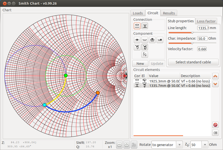
The orange dot show the antenna impedance at its feed point, the cyan dot the impedance seen through a 1925.3mm lenght coax cable, and the green dot after attaching a coax cable stub short circuited at the far end and the length 1335.7mm.
The blue circle is the g=1 circle, and the green circle is the SWR=2 circle. Also note that the colors for the dots and circles are used inconsistently among the different charts.
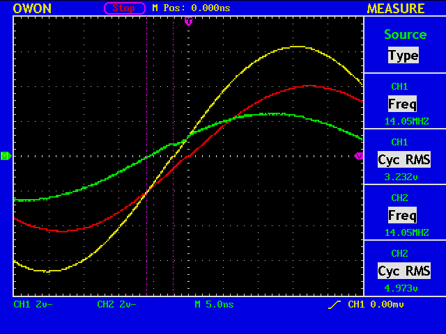
SWR-Power Meter
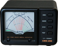
At 14.05MHz, my swr-power meter, Comet CMX-200, says that when I set
the forward power to be 6W, the reflected power becomes 2W, which means abs(gamma)=sqrt(2/6)=0.577 and swr=(1+abs(gamma))/(1-abs(gamma))=3.73.
These values are in good agreement with the ones obtained by an impedance bridge.
gnuplot> load "gnuplot1.g"
Freq [MHz]=14.05
V1=3.232
V2=4.973
Cursor 1=2.2e-009
Cursor 2=6e-009

vratio=1.53867574257426
phase1 [deg]=11.1276
phase2 [deg]=30.348

abs(gamma)=0.589937579394383
swr=3.87730623314914
cz={99.2259973692051, 90.3894587505872}
Note that the measured impedance of 99.22+i90.38 means that the impedance of the antenna at its feed point is 106.58-i90.41, considering the coax cable length of 20m.
At 18.1MHz, CMX-200 tells the forward power of 6W and the reflected power of 2.8W, which means abs(gamma)=sqrt(2.8/6)=0.683 and swr=5.31, while they are 0.688 and 5.41, respectively, by an impedance bridge.
Gnuplot and antenna
A gnuplot program for antenna impedance measurement.
# gnuplot_antenna1.g
set object 1 rectangle from screen 0,0 to screen 1,1 fillcolor rgb "#f0f0f0" behind
set size square
set xrange[-0.5:2.5]
set yrange[-1.5:1.5]
set zeroaxis
set parametric
# input data from measurement
freq=18.10e6
v1=2.422
v2=2.403
cursor1=-6.2e-9
cursor2=-16.40e-9
#
vratio=v2/v1
period=1/freq
phase1=2.0*pi*(cursor1/period)
phase2=2.0*pi*(cursor2/period)
phasedeg1=360*(cursor1/period)
phasedeg2=360*(cursor2/period)
#
I={0,1}
z0=50.0
cv1=1+I*0;
cv2=vratio*(cos(phase1)+I*sin(phase1))
cvfwd=cv1
cvrfl=cv2-cv1
cvr=2*cv1-cv2
cz=z0*(cv2/cvr)
gamma=cvrfl/cvfwd
swr=(1+abs(gamma))/(1-abs(gamma))
#
print "Freq [MHz]=", freq/1e6
print "V1=", v1
print "V2=", v2
print "Cursor 1=", cursor1
print "Cursor 2=", cursor2
print ""
print "vratio=", vratio
print "phase1 [deg]=", phasedeg1
print "phase2 [deg]=", phasedeg2
print ""
print "abs(gamma)=", abs(gamma)
print "swr=", swr
print "cz=", cz
#
set arrow 1 from 0,0 to 1,0 lw 2 lt 1
set arrow 2 from 0,0 to 2,0 lw 1 lt -1
set arrow 3 from 0,0 to real(cv2),imag(cv2) lw 2 lt 6
set arrow 4 from 1,0 to real(cv2),imag(cv2) lw 2 lt 2
set arrow 5 from real(cv2),imag(cv2) to 2,0 lw 2 lt 3
plot [0:2*pi] 1+abs(gamma)*cos(t),abs(gamma)*sin(t) lw 1 lt -1 notitle
pause -1
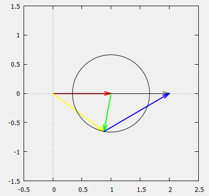
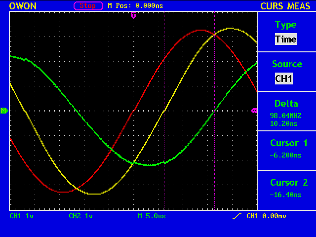
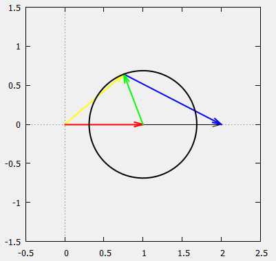
The input data comes from the following measurement.
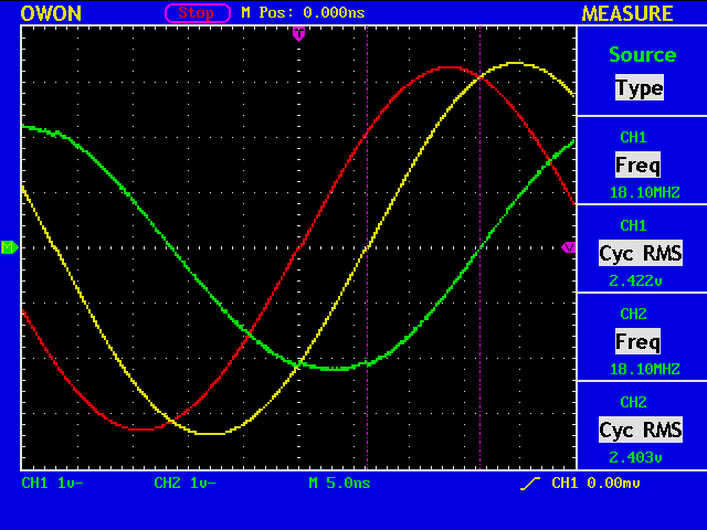
You will get the vector diagram which is essentially equivalent to the waveform observed in the above measurement.
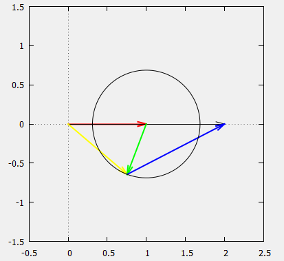
gnuplot> load "gnuplot_antenna1.g"
Freq [MHz]=18.1
V1=2.422
V2=2.403
Cursor 1=-6.2e-009
Cursor 2=-1.64e-008

vratio=0.99215524360033
phase1 [deg]=-40.3992
phase2 [deg]=-106.8624

abs(gamma)=0.687913963050921
swr=5.40848920878291
cz={13.4238815578089, -32.7726324246538}
Note: The vectors rotate counter clockwise now, which is the usual way.
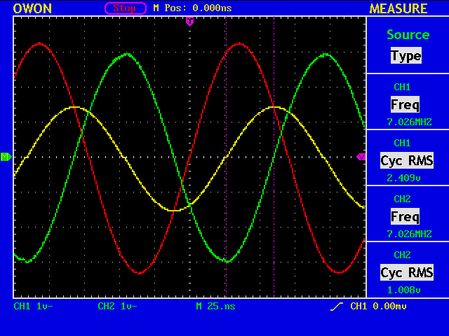
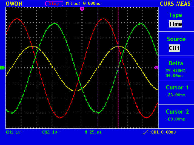
The same antenna, but at 7026kHz.
gnuplot> load "gnuplot1.g"
Freq [MHz]=7.026
V1=2.409
V2=1.008
Cursor 1=-2.6e-008
Cursor 2=-6e-008

vratio=0.418430884184309
phase1 [deg]=-65.76336
phase2 [deg]=-151.7616

abs(gamma)=0.911892223096004
swr=21.6994718318594
cz={2.414737225654, -10.9388852579521}
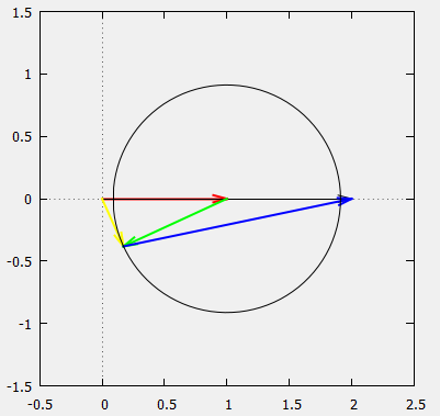
At 14.05MHz.
gnuplot> load "gnuplot1.g"
Freq [MHz]=14.05
V1=3.232
V2=4.973
Cursor 1=2.2e-009
Cursor 2=6e-009

vratio=1.53867574257426
phase1 [deg]=11.1276
phase2 [deg]=30.348

abs(gamma)=0.589937579394383
swr=3.87730623314914
cz={99.2259973692051, 90.3894587505872}
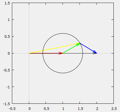
At 21.05MHz.
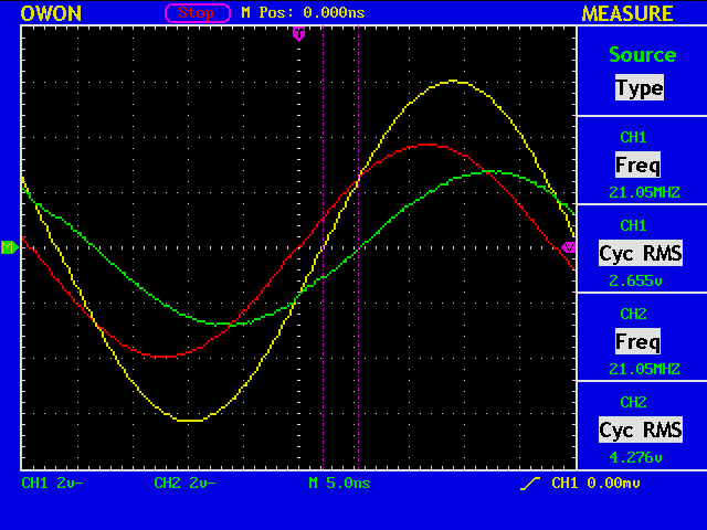
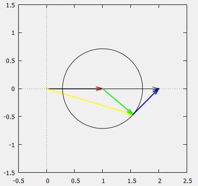
gnuplot> load "gnuplot1.g"
Freq [MHz]=21.05
V1=2.655
V2=4.276
Cursor 1=-2.2e-009
Cursor 2=-5.4e-009

vratio=1.6105461393597
phase1 [deg]=-16.6716
phase2 [deg]=-40.9212

abs(gamma)=0.712857489820842
swr=5.96518254560124
cz={58.2089871070879, -109.366273055574}
Dipole Antenna (4)
Using the same elements and a cable, a 18MHz dipole is moved slightly in its position.
The voltage ratio V2/V1=2.403/2.422=0.992, and the delay of V2 against V1 is 40.4deg (=360deg*6.20nS/55.2nS).
(%i) V1:1.0+%i*0.0;
(%i) t:2.0*3.1416*(-40.4/360.0);
(%i) V2:0.992*(cos(t)+%i*sin(t));
(%i) Vr:2*V1-V2;
(%i) z:50.0*V2/Vr;
(%i) realpart(z);
(%o) 13.42379132002304
(%i) imagpart(z);
(%o) -32.76468187626101
(%i) abs(z);
(%o) 35.40794475617177
(%i) g:(z-50)/(z+50);
(%i) abs(g);
(%o) 0.6878765282155
(%i) SWR:(1+abs(g))/(1-abs(g));
(%o) 5.407720600329899
gnuplot> set object 1 rectangle from screen 0,0 to screen 1,1 fillcolor rgb "#f0f0f0" behind
gnuplot> set size square
gnuplot> set xrange[-0.5:2.5]
gnuplot> set yrange[-1.5:1.5]
gnuplot> set zeroaxis
gnuplot> set parametric
gnuplot> plot [0:2*pi] 1+cos(t)*0.6878,sin(t)*0.6878 lw 2 lt -1 notitle
gnuplot> set arrow 3 from 0,0 to 0.992*cos(40.4/360.0*2.0*3.1416),0.992*sin(40.4/360.0*2.0*3.1416) lw 2 lt 6
The same antenna, but at 7026kHz.
The voltage ratio V2/V1=1.008/2.409=0.418, and the delay of V2 against V1 is 65.8deg (=360deg*26.0nS/142.3nS).
(%i) V1:1.0+%i*0.0;
(%i) t:2.0*3.1416*(-65.8/360.0);
(%i) V2:0.418*(cos(t)+%i*sin(t));
(%i) Vr:2*V1-V2;
(%i) z:50.0*V2/Vr;
(%i) realpart(z);
(%o) 2.40689877387539
(%i) imagpart(z);
(%o) -10.92662280617141
(%i) abs(z);
(%o) 11.18857665907635
(%i) g:(z-50)/(z+50);
(%i) abs(g);
(%o) 0.91215699937376
(%i) SWR:(1+abs(g))/(1-abs(g));
(%o) 21.76789255537643
Matching Impedances
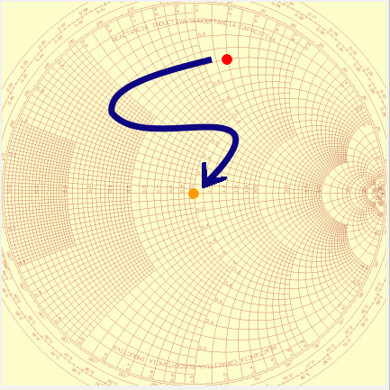
Suppose your antenna has some strange impedance of, say, Zant=20+i60 ohm (red dot). Then, you need to do something so that the impedance seen from the transmitter becomes, at least close enough to, Z0=50+i0 ohm (orange dot).
This can be done in several different ways, but one thing worth remembering is that the impedance itself, Zant=20+i60 ohm in this case, is not very essential, although this is the value you observe with an antenna analyzer when it is attached to the feeding point of your antenna.
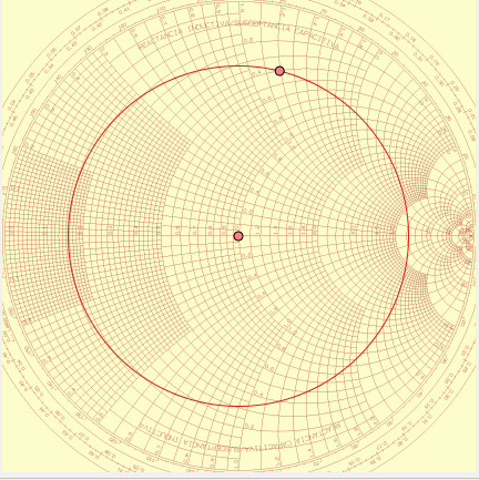
More essential is the constant gamma circle (red) on which the various impedances you will observe through a different length of a coax cable will all appear.
Note: The gamma=(Zant-Z0)/(Zant+Z0), abs(gamma)=0.7276,
and VSWR=(1+abs(gamma)) / (1-abs(gamma))=6.342.
By varying the cable length, the reactance, the imaginary part of the impedance, becomes either inductive (upper half of the plane) or capacitive (the lower half of the plane), or the impedance be purely resistive (on the X=0 axis).
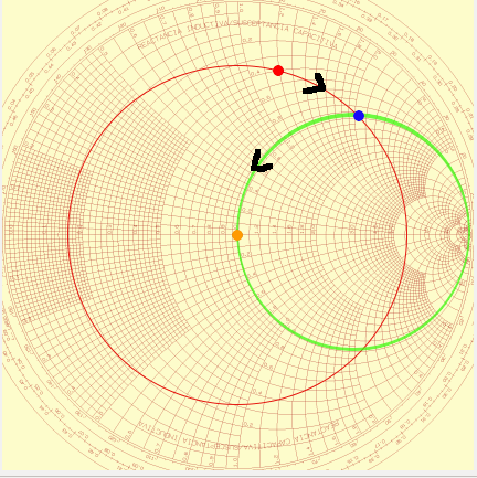
Now, one more step to go from the red dot to the orange dot.
Starting form the red dot, you can select any point on the red circle by changing the cable length, and since you only wish to use purely reactive devices for your impedance matching network to avoid any power loss, you are moving on the green circle on which the R is 50 ohm everywhere, to reach your destination, the orange dot.
These two circles, red and green, will determine the mid-point (blue dot), to where you will move from the red dot, and from where you will move to the orange dot.
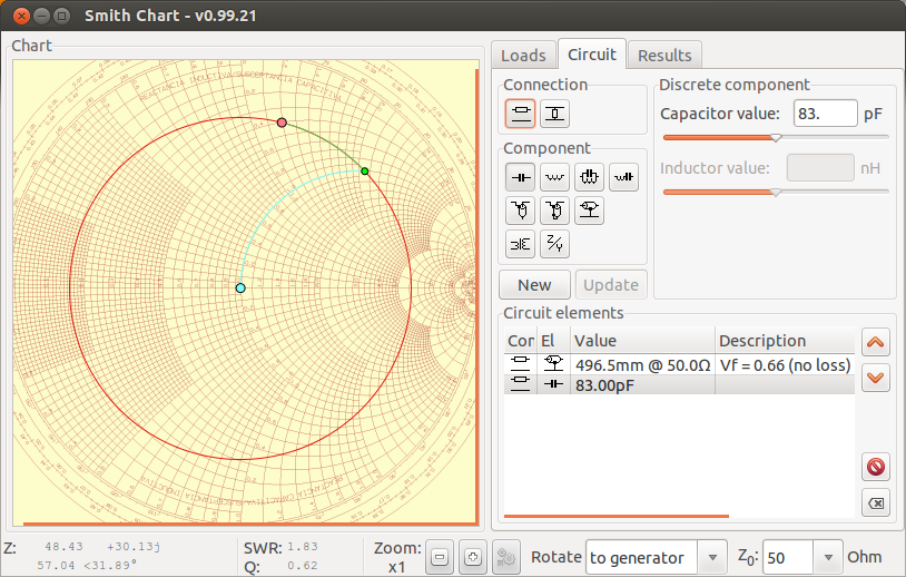
One example is shown here. With the frequency of 18.1MHz, the cable lenght of 496.5mm will bring you from the red dot (Zant=20+i60 ohm) to the green dot (Zmid=50+i106 ohm), and the series capacitance of 83pF (Zc=-i106 ohm) at the near end of the cable will bring you from the green dot to the cyan dot (Z0=50 ohm). (The coloring differs, but you will understand.)
Then, you can use a cable of any length to connect your transmitter and the 83pF capacitance + 496.5mm cable + your antenna.
LTspice Device Model (3)
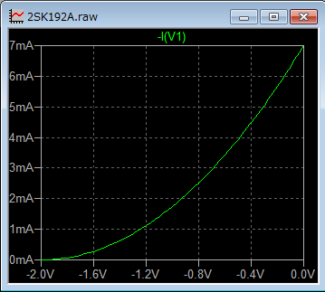
Now, we measure the actual device parameters. Here is a circuit with a single voltage source. We vary the value of R1 to get the Id=Id(Vg) curve.
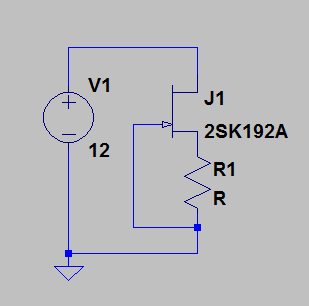
I used a 100 ohm and a 1k ohm resistors for R1. The lord lines are in orange (-2V gives 20mA) and in blue (-4V gives 4mA) in the figure, and the measured values, -0.44V for a 100 ohm resistor and -1.21V for a 1k ohm resistor, are plotted in red.
The Idss classification for the device is GR (6.0-14.0mA), shown in green in the figure, and we conclude that the Idss=7mA and the Vto=-2V is a good guess.
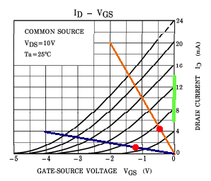
The Beta is obtained from the equation, Beta=Idss/(Vto^2)=7m/(-2)^2=1.75m, to give the device model of;
.model 2SK192A NJF(beta=1.75m vto=-2.0 cgd=1p cgs=2p)
and the following Id=Id(Vg) curve.
If we choose Id to be 3mA, R4 now becomes (6V-(-0.7V))/3mA~2kohm.
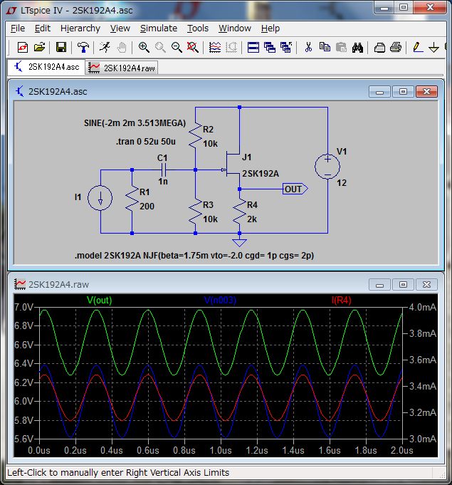
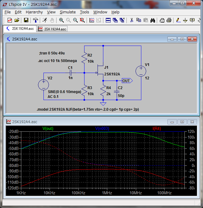
In AC analysis, a relatively large stray capacity of 50nF is assumed.
LTspice Device Model (2)
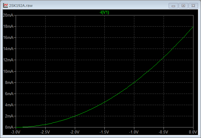
Something I forgot to mention in my previous post. The drain current Id is a function of the gate-source voltage Vg, namely Id=Id(Vg). Idss is defined as Id(0), and Vto is the voltage such that Id(Vto)=0. It is easy to measure these two parameters, Idss and Vto, if you have a device, but what you need for your device model is Beta and Vto, not Idss and Vto.
If you know the parameters Idss and Vto, you can express the drain current as Id=Idss*(1-(Vg/Vto))^2. Or if you know Beta and Vto, Id=Beta*(Vg-Vto)^2. Of course these two equations are equivalent, therefore you have Beta=Idss/(Vto^2), or Idss=Beta*(Vto)^2.
In the above example, the model is
.model 2SK192A NJF(beta=2.0m vto=-3.0 cgd=1p cgs=2p)
This model gives Idss=2.0m*(-3.0)^2=18m [A], as you can see from the figure.
And just one more thing..
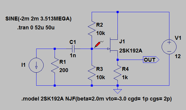
A very simple design method for a source follower. You only need to decide three parameters, R2, R3 and R4. First, let R2=R3 so that the DC operating point is around Vdd/2(=6V). Next, you decide the Id. Looking at the Id=Id(Vg) curve, you choose Id=8mA and this gives Vg=-1.0V, which means R4=(6V-(-1V))/8mA~1kohm.
Since the source impedance is only 200ohm in this particular example, R2 and R3 could be anything, say 10kohm.
Finally, C1 should be small enough compared with R2//R3 at the operating frequency, so let C1 be 1nF, equivalent to 50ohm around 3.5MHz.