
A gnuplot program for antenna impedance measurement.
# gnuplot_antenna1.g
set object 1 rectangle from screen 0,0 to screen 1,1 fillcolor rgb "#f0f0f0" behind
set size square
set xrange[-0.5:2.5]
set yrange[-1.5:1.5]
set zeroaxis
set parametric
# input data from measurement
freq=18.10e6
v1=2.422
v2=2.403
cursor1=-6.2e-9
cursor2=-16.40e-9
#
vratio=v2/v1
period=1/freq
phase1=2.0*pi*(cursor1/period)
phase2=2.0*pi*(cursor2/period)
phasedeg1=360*(cursor1/period)
phasedeg2=360*(cursor2/period)
#
I={0,1}
z0=50.0
cv1=1+I*0;
cv2=vratio*(cos(phase1)+I*sin(phase1))
cvfwd=cv1
cvrfl=cv2-cv1
cvr=2*cv1-cv2
cz=z0*(cv2/cvr)
gamma=cvrfl/cvfwd
swr=(1+abs(gamma))/(1-abs(gamma))
#
print "Freq [MHz]=", freq/1e6
print "V1=", v1
print "V2=", v2
print "Cursor 1=", cursor1
print "Cursor 2=", cursor2
print ""
print "vratio=", vratio
print "phase1 [deg]=", phasedeg1
print "phase2 [deg]=", phasedeg2
print ""
print "abs(gamma)=", abs(gamma)
print "swr=", swr
print "cz=", cz
#
set arrow 1 from 0,0 to 1,0 lw 2 lt 1
set arrow 2 from 0,0 to 2,0 lw 1 lt -1
set arrow 3 from 0,0 to real(cv2),imag(cv2) lw 2 lt 6
set arrow 4 from 1,0 to real(cv2),imag(cv2) lw 2 lt 2
set arrow 5 from real(cv2),imag(cv2) to 2,0 lw 2 lt 3
plot [0:2*pi] 1+abs(gamma)*cos(t),abs(gamma)*sin(t) lw 1 lt -1 notitle
pause -1
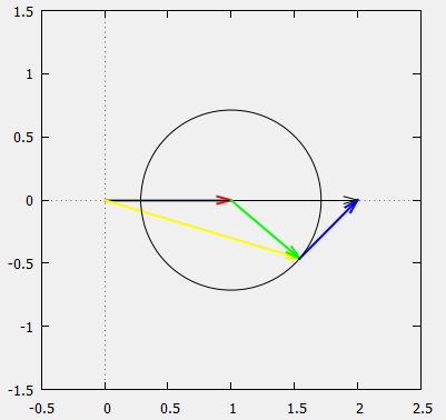
The input data comes from the following measurement.
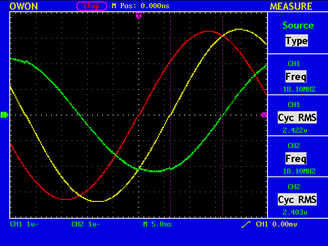
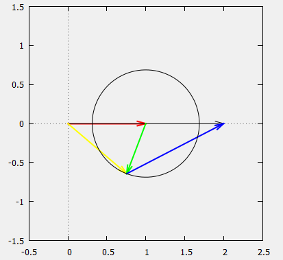
You will get the vector diagram which is essentially equivalent to the waveform observed in the above measurement.
gnuplot> load "gnuplot_antenna1.g"
Freq [MHz]=18.1
V1=2.422
V2=2.403
Cursor 1=-6.2e-009
Cursor 2=-1.64e-008

vratio=0.99215524360033
phase1 [deg]=-40.3992
phase2 [deg]=-106.8624

abs(gamma)=0.687913963050921
swr=5.40848920878291
cz={13.4238815578089, -32.7726324246538}
Note: The vectors rotate counter clockwise now, which is the usual way.
The same antenna, but at 7026kHz.
gnuplot> load "gnuplot1.g"
Freq [MHz]=7.026
V1=2.409
V2=1.008
Cursor 1=-2.6e-008
Cursor 2=-6e-008

vratio=0.418430884184309
phase1 [deg]=-65.76336
phase2 [deg]=-151.7616

abs(gamma)=0.911892223096004
swr=21.6994718318594
cz={2.414737225654, -10.9388852579521}
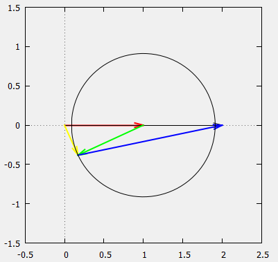
At 14.05MHz.
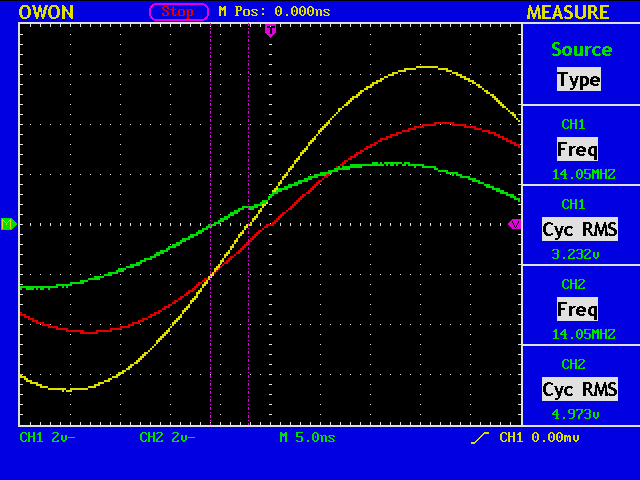
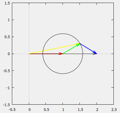
gnuplot> load "gnuplot1.g"
Freq [MHz]=14.05
V1=3.232
V2=4.973
Cursor 1=2.2e-009
Cursor 2=6e-009

vratio=1.53867574257426
phase1 [deg]=11.1276
phase2 [deg]=30.348

abs(gamma)=0.589937579394383
swr=3.87730623314914
cz={99.2259973692051, 90.3894587505872}
At 21.05MHz.
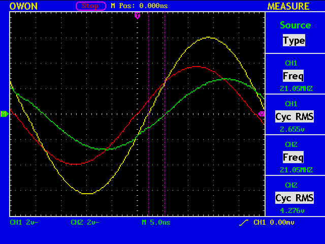
gnuplot> load "gnuplot1.g"
Freq [MHz]=21.05
V1=2.655
V2=4.276
Cursor 1=-2.2e-009
Cursor 2=-5.4e-009

vratio=1.6105461393597
phase1 [deg]=-16.6716
phase2 [deg]=-40.9212

abs(gamma)=0.712857489820842
swr=5.96518254560124
cz={58.2089871070879, -109.366273055574}