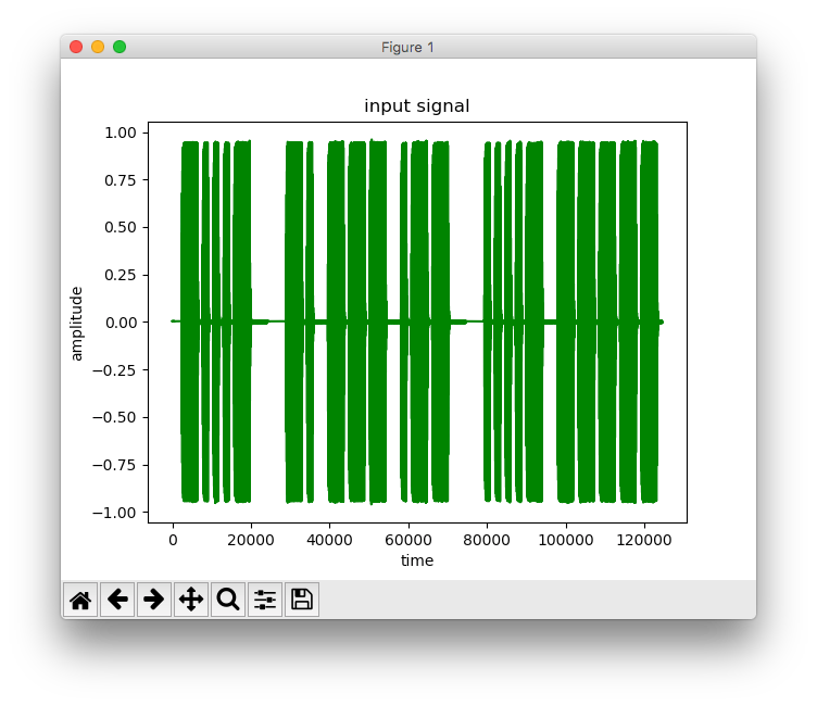
$ ~/anaconda3/bin/python test4.py ~/40wpm.wav 0 -1

<BT>
NOW
40
WPM
<BT>
TEXT
IS
FROM
JANUARY
2014
QST
PAGE
46
<BT>
SETTING
THE
VFO.
WITH
THE
TRANSMITTER
OUTPUT
CONNECTED
TO
A
DUMMY
LOAD,
SET
THE
VFO
TO
THE
CORRECT
FREQUENCY
FOR
THE
BAND
OF
INTEREST.
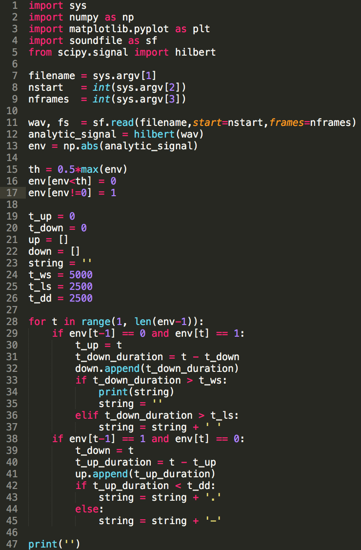
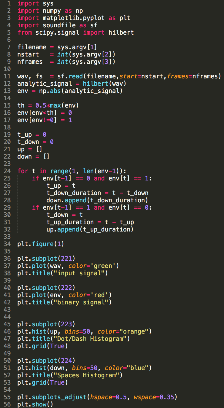
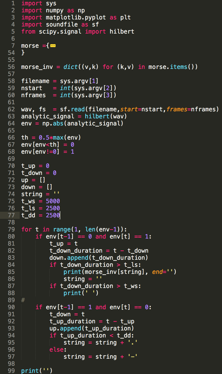
import sys
import numpy as np
import matplotlib.pyplot as plt
import soundfile as sf
from scipy.signal import hilbert
morse ={
"" : "",
"A" : ".-",
"B" : "-...",
"C" : "-.-.",
"D" : "-..",
"E" : ".",
"F" : "..-.",
"G" : "--.",
"H" : "....",
"I" : "..",
"J" : ".---",
"K" : "-.-",
"L" : ".-..",
"M" : "--",
"N" : "-.",
"O" : "---",
"P" : ".--.",
"Q" : "--.-",
"R" : ".-.",
"S" : "...",
"T" : "-",
"U" : "..-",
"V" : "...-",
"W" : ".--",
"X" : "-..-",
"Y" : "-.--",
"Z" : "--..",
"1" : ".----",
"2" : "..---",
"3" : "...--",
"4" : "....-",
"5" : ".....",
"6" : "-....",
"7" : "--...",
"8" : "---..",
"9" : "----.",
"0" : "-----",
"." : ".-.-.-",
"," : "--..--",
":" : "---...",
"?" : "..--..",
"'" : ".----.",
"-" : "-....-",
"/" : "-..-.",
"@" : ".--.-.",
"<BT>" : "-...-"
}
morse_inv = dict((v,k) for (k,v) in morse.items())
filename = sys.argv[1]
nstart = int(sys.argv[2])
nframes = int(sys.argv[3])
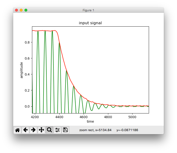
wav, fs = sf.read(filename,start=nstart,frames=nframes)
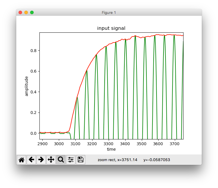
analytic_signal = hilbert(wav)
env = np.abs(analytic_signal)
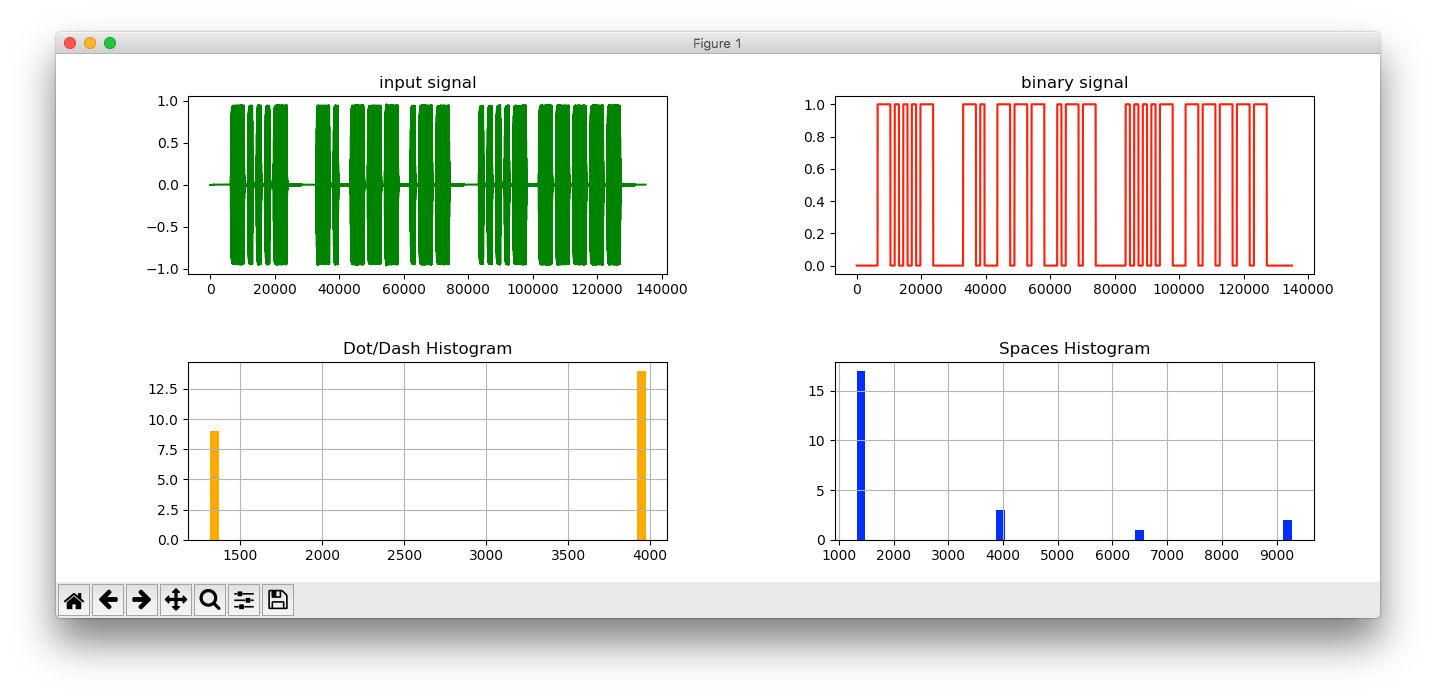
th = 0.5*max(env)
env[env<th] = 0
env[env!=0] = 1
t_up = 0
t_down = 0
up = []
down = []
string = ''
t_ws = 5000
t_ls = 2500
t_dd = 2500
for t in range(1, len(env-1)):
if env[t-1] == 0 and env[t] == 1:
t_up = t
t_down_duration = t - t_down
down.append(t_down_duration)
if t_down_duration > t_ls:
print(morse_inv[string], end='')
string = ''
if t_down_duration > t_ws:
print(' ')
if env[t-1] == 1 and env[t] == 0:
t_down = t
t_up_duration = t - t_up
up.append(t_up_duration)
if t_up_duration < t_dd:
string = string + '.'
else:
string = string + '-'
print('')