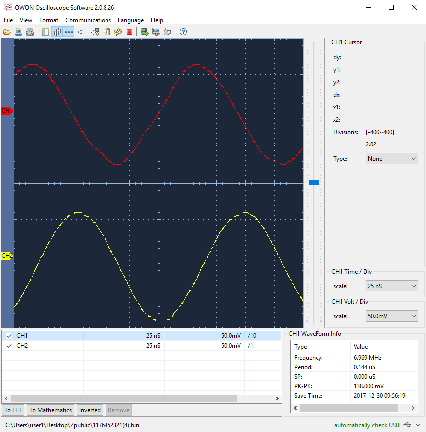
Now, with a frequency mixer, TAK-5.

LO: 12.5MHz, RF: 5MHz.
LO: 12.5MHz, RF: 7.5Mhz.

LO: 15MHz, RF: 5MHz.

Ham Radio Blog
Now, with a frequency mixer, TAK-5.
LO: 12.5MHz, RF: 5MHz.
LO: 12.5MHz, RF: 7.5Mhz.
LO: 15MHz, RF: 5MHz.
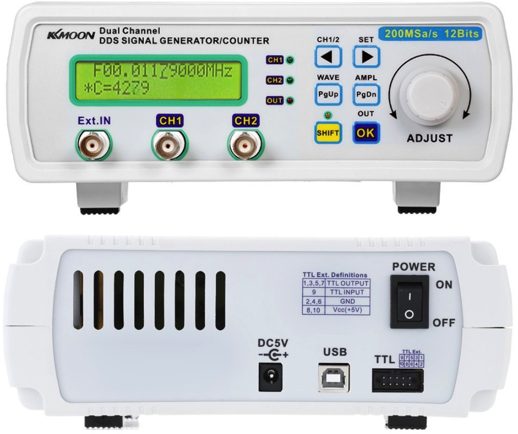
This is a very low-cost signal generator I recently acquired.

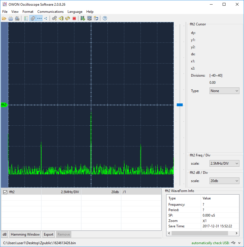
Let’s do some experiment with a power splitter/combiner, PSCQ-2-7.5.
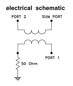
First, as a splitter:
A signal around 7MHz is applied to the sum port, and the output signals from port 1 and port 2 are observed. The phase difference of the two signals should be 90 deg.
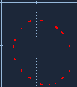
Next, as a combiner.
Two signals with the frequency of 7010kHz and 7110kHz are applied to the port A and the port B, respectively.
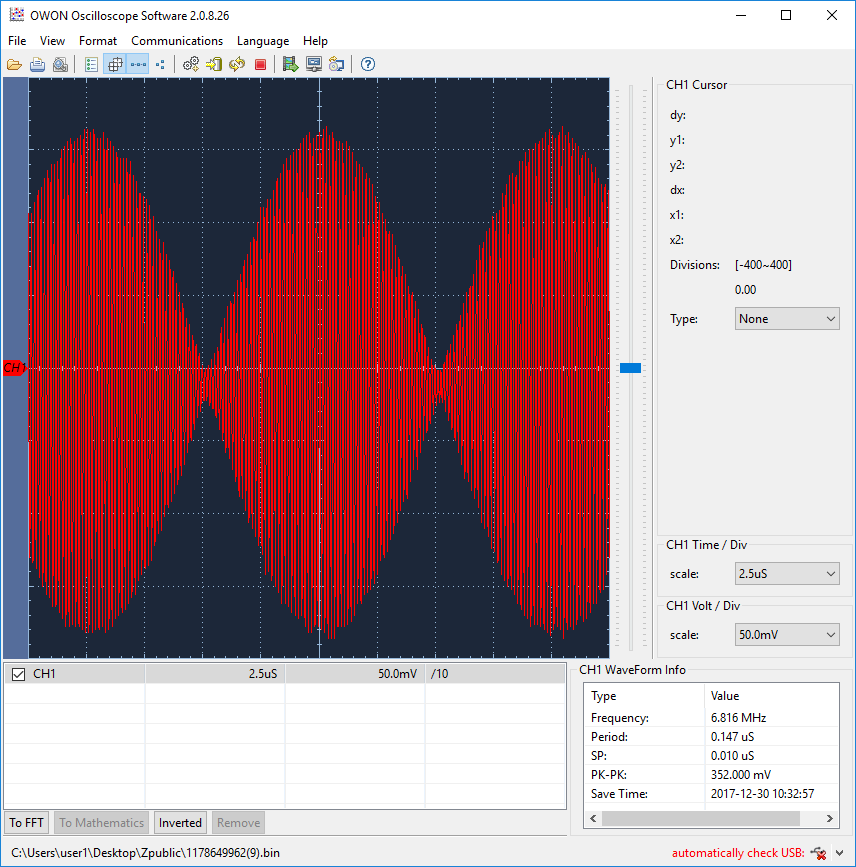
This is what is observed at the sum port.

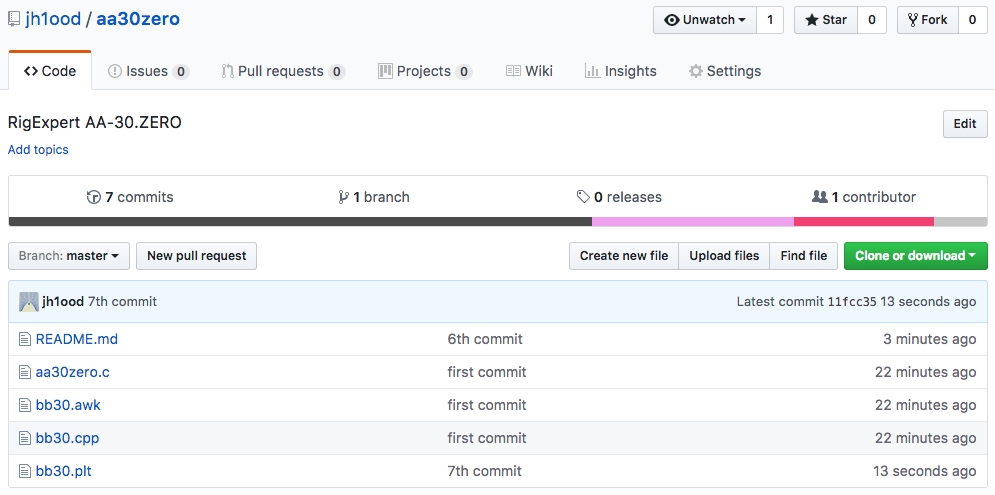
Did some minor improvement to the software. Please visit my new page, AA-30.ZERO for the latest version of the programs.
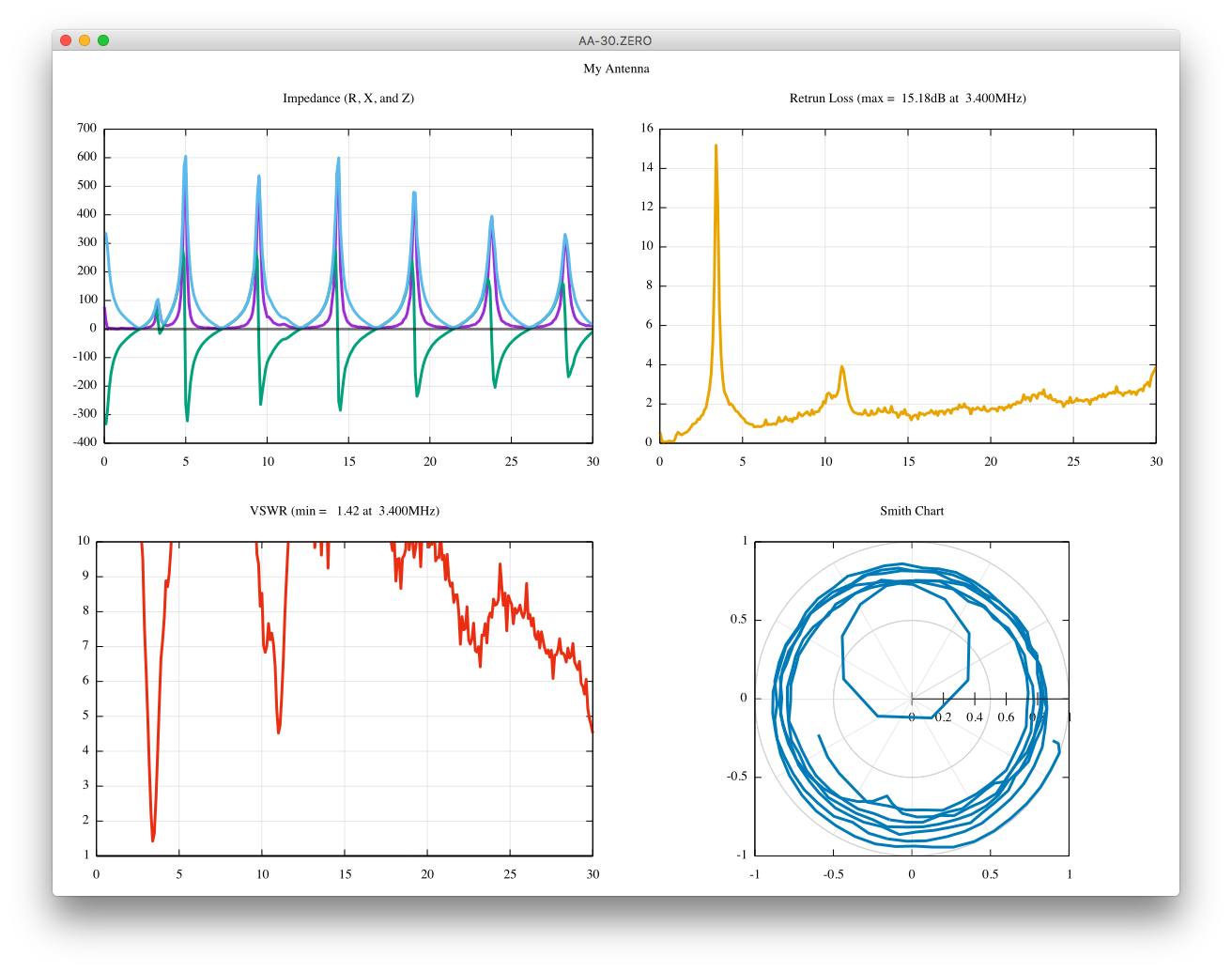
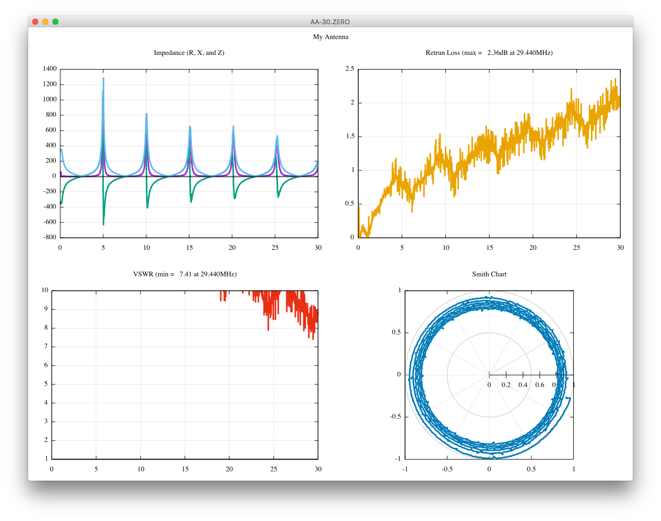
I am using a 20m coaxial cable (5D-2V) and its far end is left open during the measurement.
The Smith Chart tells you everything, but it is easier to see its amplitude and phase separately.
First, the amplitude in dB.
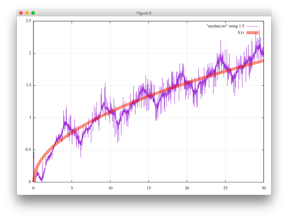
% gnuplot
gnuplot> f(x)=a*sqrt(x)
gnuplot> fit f(x) "mydata.txt" using 1:5 via a
iter      chisq       delta/lim  lambda   a
   0 9.0593050625e+02   0.00e+00  8.02e-01    2.070472e-01
   1 5.4539304323e+01  -1.56e+06  8.02e-02    3.445278e-01
   2 5.4539209850e+01  -1.73e-01  8.02e-03    3.445736e-01
iter      chisq       delta/lim  lambda   a

After 2 iterations the fit converged.
final sum of squares of residuals : 54.5392
rel. change during last iteration : -1.7322e-06

degrees of freedom    (FIT_NDF)                        : 3000
rms of residuals      (FIT_STDFIT) = sqrt(WSSR/ndf)    : 0.134832
variance of residuals (reduced chisquare) = WSSR/ndf   : 0.0181797

Final set of parameters            Asymptotic Standard Error
=======================            ==========================
a               = 0.344574         +/- 0.0006355    (0.1844%)
gnuplot> print a*sqrt(30)
1.88730727013936
The loss of 1.887[dB] at 30MHz agrees well with its nominal value of 0.44dB/10m, or 1.76dB/40m.
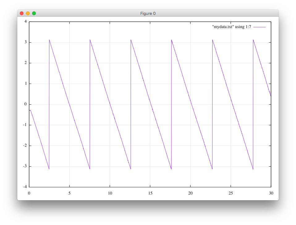
Next, the phase in radian.
 .
.
Let’s see at which frequencies the phase changes from -pi to +pi.
 2.48, 1.3514, -0.299513, 1.3842, 0.469624, 36.9999, -3.1296, 0.947368
 2.49, 1.39451, 0.083306, 1.397, 0.484627, 35.8549, 3.13826, 0.945733

 7.53, 2.59869, -0.289392, 2.61476, 0.903662, 19.2411, -3.12999, 0.901191
 7.54, 2.45728, 0.08333, 2.4587, 0.854434, 20.3477, 3.13825, 0.906313

 12.6, 3.4673, -0.351551, 3.48508, 1.20654, 14.4212, -3.12746, 0.870308
 12.61, 3.43064, 0.097069, 3.43201, 1.1938, 14.5746, 3.13769, 0.871586
...
 27.77, 5.43172, -0.091826, 5.43249, 1.89464, 9.20522, -3.13788, 0.804022
 27.78, 5.31208, 0.100171, 5.31302, 1.85259, 9.41255, 3.13754, 0.807924
The period is (27.77MHz-2.48MHz)/5cyles, which is 5.06MHz/cycle.
The electrical length of the cable is thus (300m*MHz/5.06MHz)/2=29.64m.
Assuming the velocity factor of 66%, the physical length is known to be 19.56m.
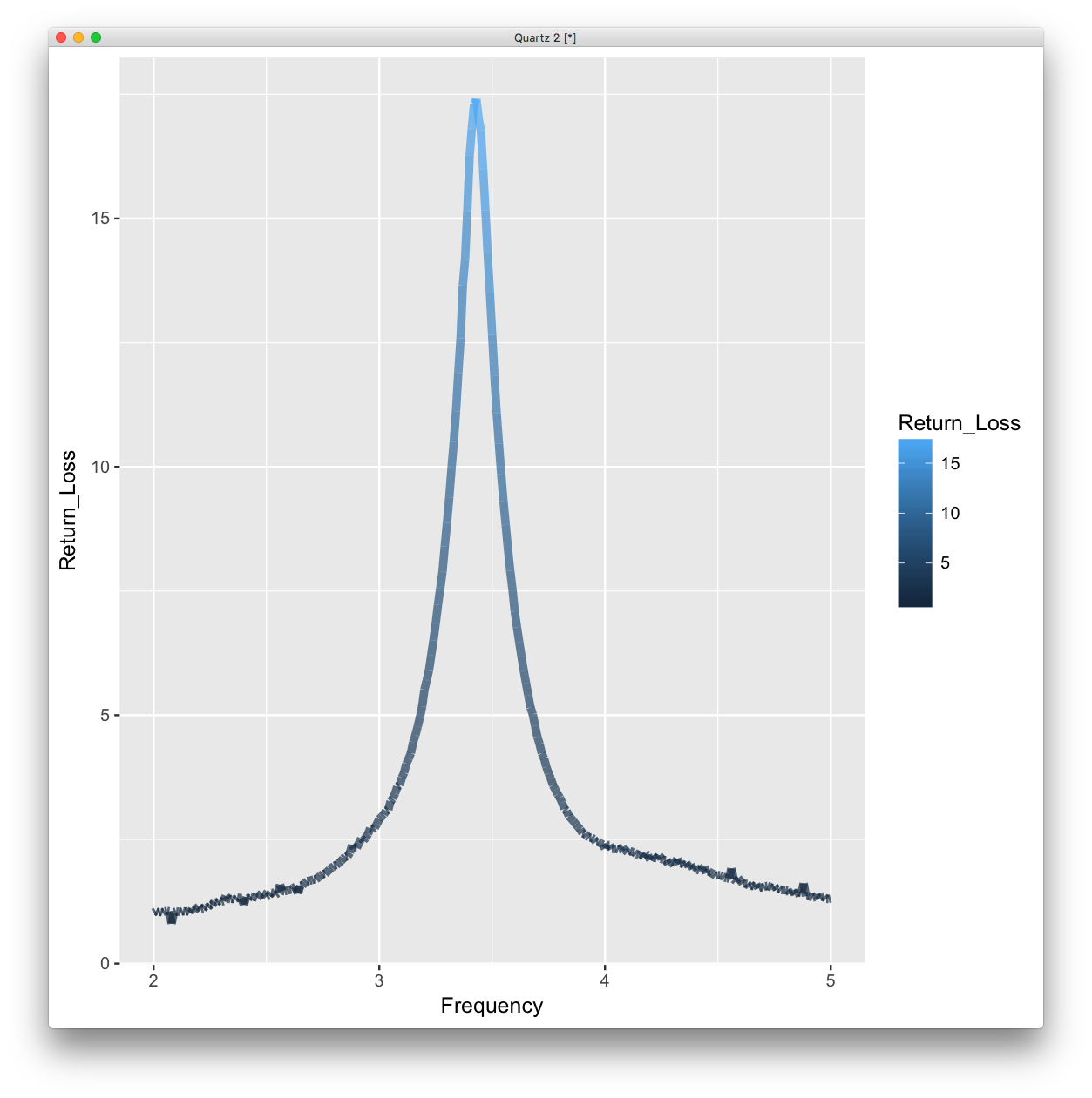
Using ggplot2 is another way to plot a graph with R.
% head mydataR.txt
Frequency, R, X, Z, Return_Loss, VSWR, rhoAng, rhoAbs
2, 2.99567, -6.27359, 6.95212, 1.0258, 16.9545, -2.89108, 0.888607
2.01, 3.07187, -5.98362, 6.72608, 1.05344, 16.5107, -2.9025, 0.885784
2.02, 3.00247, -5.64513, 6.39393, 1.0312, 16.866, -2.91594, 0.888055
...
% R
> data<-read.table("mydataR.txt",sep=",",header=T)
> gp = ggplot(data, aes(x=Frequency, y=Return_Loss, colour=Return_Loss))
> gp = gp + geom_line(size=2, alpha=0.7)
> print(gp)
You can also use R for plotting.
% R
> data<-read.table("mydata.txt",sep=",")
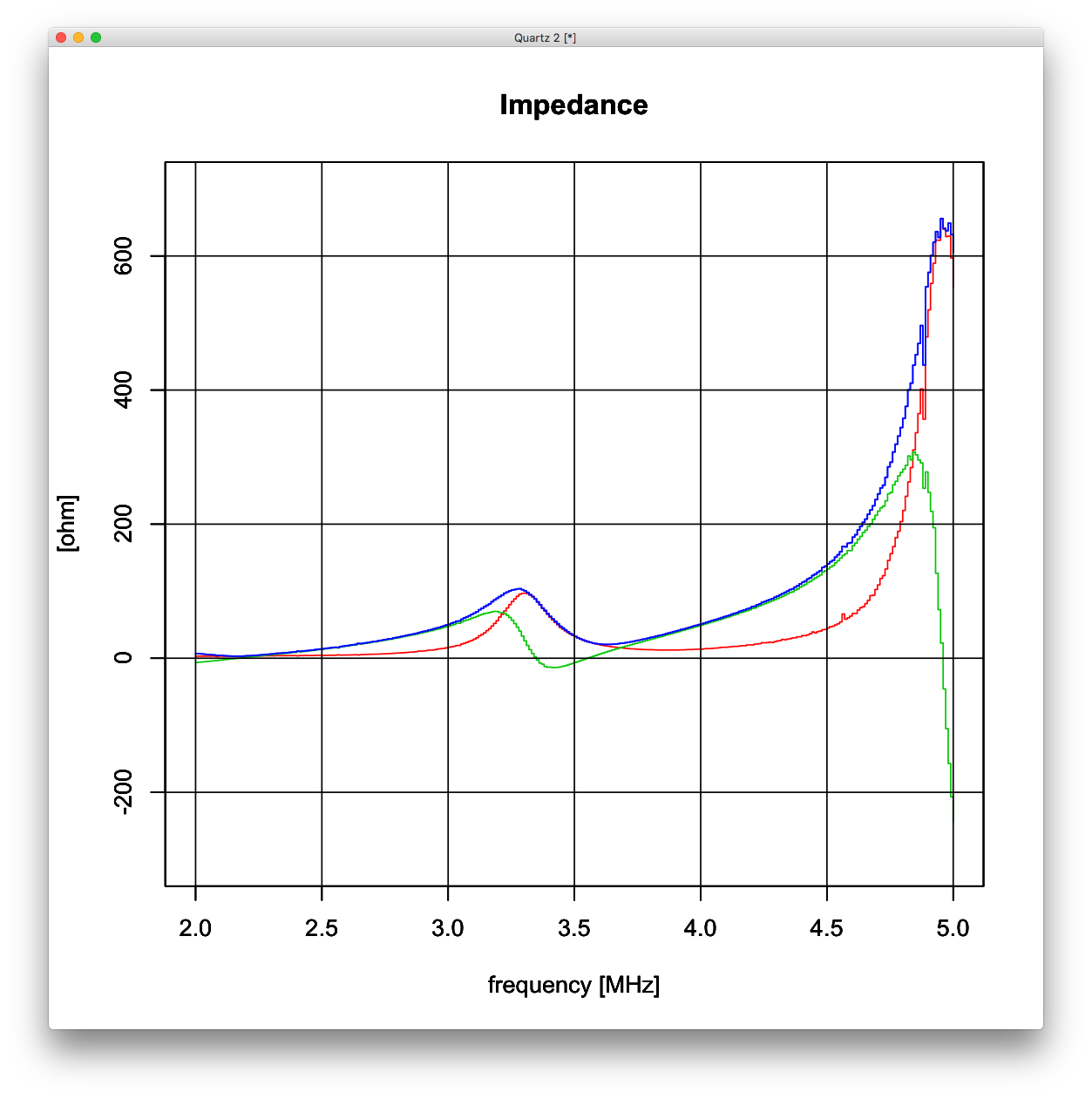
> plot(x=data$V1, y=data$V2, type="s", main="Impedance", xlab="frequency [MHz]", ylab="[ohm]", ylim=c(-300,700), col=2)
> par(new=T)
> plot(x=data$V1, y=data$V3, type="s", main="Impedance", xlab="frequency [MHz]", ylab="[ohm]", ylim=c(-300,700), col=3)
> par(new=T)
> plot(x=data$V1, y=data$V4, type="s", main="Impedance", xlab="frequency [MHz]", ylab="[ohm]", ylim=c(-300,700), col=4, tck=1)
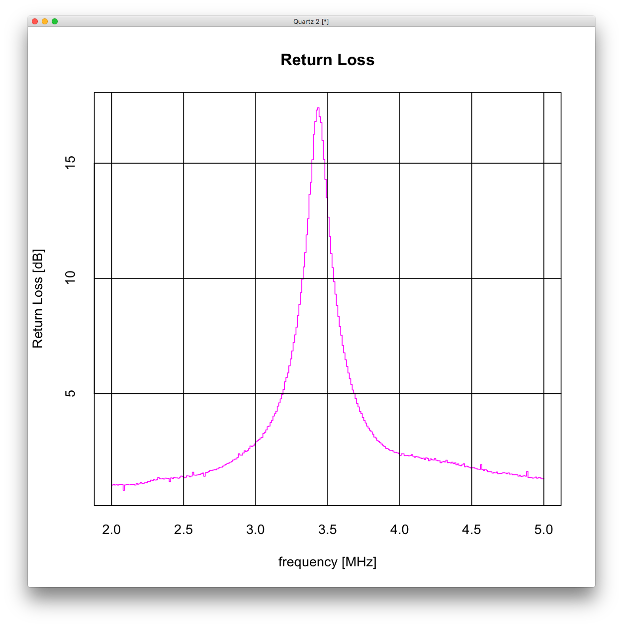
> plot(x=data$V1, y=data$V5, type="s", main="Return Loss", xlab="frequency [MHz]", ylab="Return Loss [dB]", col=6, tck=1)
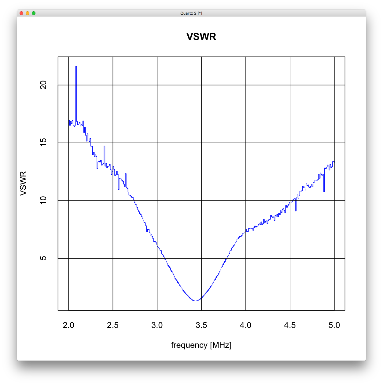
> plot(x=data$V1, y=data$V6, type="s", main="VSWR", xlab="frequency [MHz]", ylab="VSWR", col=4, tck=1)
There should be a better way, but this works.
/* Data Converter for Rig Expert AA-30.ZERO */
/* % g++ bb30.cpp -o bb30 */
#include <complex>
#include <iostream>
#include <sstream>
#include <string>
using namespace std;

int main(int argc, char *argv[]) {
  string fval, rval, xval;
  double f, r, x;
  double absz, retloss, vswr;
  complex<double> z, rho;
  const complex<double> z0 = 50.0;

  while (!cin.eof()) {
    getline(cin, fval, ',');
    getline(cin, rval, ',');
    getline(cin, xval, '\n');

    stringstream(fval) >> f;
    stringstream(rval) >> r; if(r<0) r=0.01;
    stringstream(xval) >> x;

    z       = complex<double>(r,x);
    absz    = abs(z);
    rho     = (z-z0)/(z+z0);
    retloss = -20.0 * log( abs(rho) ) / log( 10.0 );
    vswr    = ( 1+abs(rho) ) / ( 1-abs(rho) );

    cout << f << ", " << r << ", " << x << ", " << absz << ", "
         << retloss << ", " << vswr << ", "
         << arg(rho) << ", " << abs(rho) << endl;
  }
}
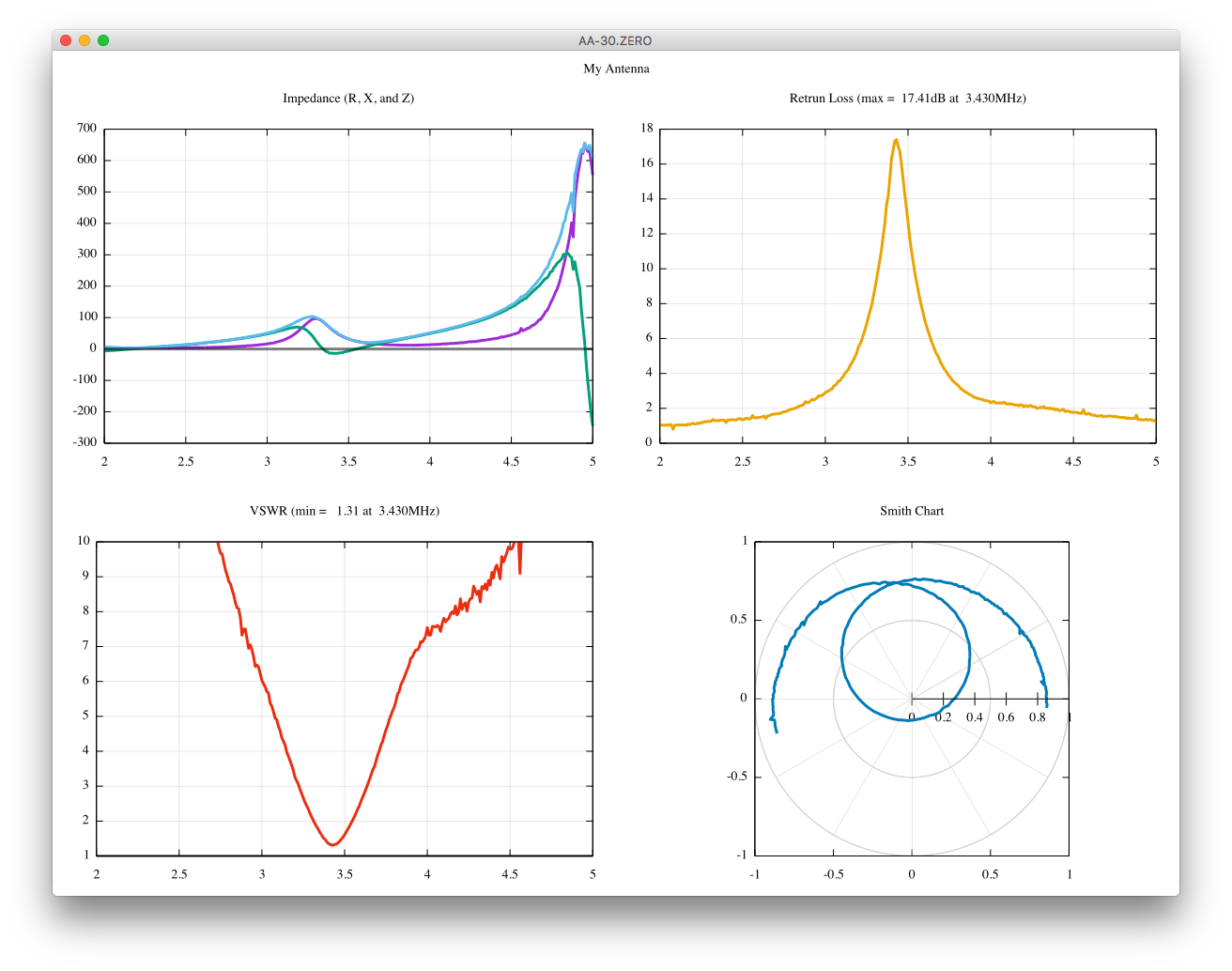
# Gnuplot script for AA-30.ZERO

reset
set terminal aqua enhanced title 'AA-30.ZERO' size 1200 900
set multiplot layout 2,2 title 'My Antenna'
set grid
unset key

fname = 'mydata.txt'
set datafile separator ','

set title 'Impedance (R, X, and Z)'
plot   fname using 1:2 with line linewidth 3, \
       ''    using 1:3 with line linewidth 3, \
       ''    using 1:4 with line linewidth 3, \
       0.0             with line linewidth 3 lc "#80000000"

stats '' using 1:5 nooutput
set title sprintf("Retrun Loss (max = %6.2fdB at %6.3fMHz)", STATS_max_y, STATS_pos_max_y)
plot '' using 1:5 with line linewidth 3 linetype 4


stats fname using 1:6 nooutput
set title sprintf("VSWR (min = %6.2f at %6.3fMHz)", STATS_min_y, STATS_pos_min_y)
set yrange [1:10]
plot '' using 1: 6 with line linewidth 3 linetype 7, \
     1.0           with line linewidth 3 lc "#80000000"

set title 'Smith Chart'
set polar
set grid polar
set size square
set xrange [-1:+1]
set yrange [-1:+1]
plot '' using 7:8 with line linewidth 3 linetype 6

unset multiplot
reset
% ./aa30zero /dev/cu.usbmodem1461 fq3500000 sw3000000 frx300 | ./bb30 > mydata.txt
This is more readable.
# Gnuplot script for AA-30.ZERO

reset
set terminal aqua enhanced title 'AA-30.ZERO' size 1200 900
set multiplot layout 2,2 title 'My Antenna'
set grid
unset key

fname = 'mydata.txt'
set datafile separator ','

z0         = 50.0
z(r,x)     = r + x*{0,1}
rho(z)     = (z-z0)/(z+z0)
retloss(z) = -20.0 * log( abs(rho(z)) ) / log( 10.0 )
vswr(z)    = ( 1+abs(rho(z)) ) / ( 1-abs(rho(z)) )

set title 'Impedance (R, X, and Z)'
plot   fname using 1:( abs(z($2,$3)) ) with line linewidth 3, \
       ''    using 1:2                 with line linewidth 3, \
       ''    using 1:3                 with line linewidth 3, \
       0.0                             with line linewidth 3 lc "#80000000"

set title 'Return Loss'
plot '' using 1:( retloss(z($2,$3)) ) with line linewidth 3 linetype 4

set title 'VSWR'
plot '' using 1:( vswr   (z($2,$3)) ) with line linewidth 3 linetype 7, \
     1.0                              with line linewidth 3 lc "#80000000"

set title 'Smith Chart'
set polar
set grid polar
set size square
set xrange [-1:+1]
plot '' using ( arg(rho(z($2,$3))) ) : ( abs(rho(z($2,$3))) ) : (3*$1) with line linewidth 3 linetype 6

unset multiplot
reset
You can draw nice graphs very easily using Gnuplot.
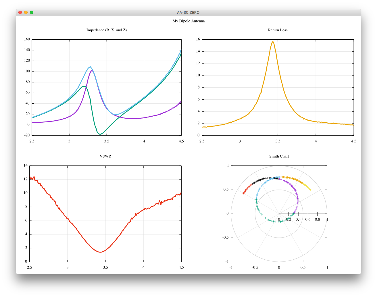
The raw data obtained from your AA-30.ZERO is:
...
2.990000,15.066906,46.652055
3.000000,15.557470,48.099209
3.010000,16.004803,48.884680
...
And the script is:
# Gnuplot script for AA-30.ZERO
reset
set terminal aqua enhanced title "AA-30.ZERO" size 1200 900
set datafile separator ","
set grid
unset key
set multiplot layout 2,2 title "My Dipole Antenna"

set title "Impedance (R, X, and Z)"
plot   "mydata.txt" using 1:2 with line linewidth 3, \
"mydata.txt" using 1:3 with line linewidth 3, \
"mydata.txt" using 1:( abs($2+$3*{0,1}) ) with line linewidth 3

set title "Return Loss"
plot "mydata.txt" using 1:( -20.0 * log(abs( ($2+$3*{0,1}-50)/($2+$3*{0,1}+50) )) / log(10) ) with line linewidth 3 linetype 4

set title "VSWR"
plot "mydata.txt" using 1:( (1+abs( ($2+$3*{0,1}-50)/($2+$3*{0,1}+50) )) / (1-abs( ($2+$3*{0,1}-50)/($2+$3*{0,1}+50) )) ) with line linewidth 3 linetype 7

set title "Smith Chart"
set polar
set grid polar
set size square
set xrange [-1:+1]
plot "mydata.txt" using (arg( ($2+$3*{0,1}-50)/($2+$3*{0,1}+50) )) : (abs( ($2+$3*{0,1}-50)/($2+$3*{0,1}+50) )) : (3*$1) with point pointtype 7 lc variable

unset multiplot
Set the terminal type properly depending on your platform. See the line 3 of the script.
Then all you have to do is:
% ./aa30zero fq3500000 sw2000000 frx200 > mydata.txt
% gnuplot aa30zero.plt