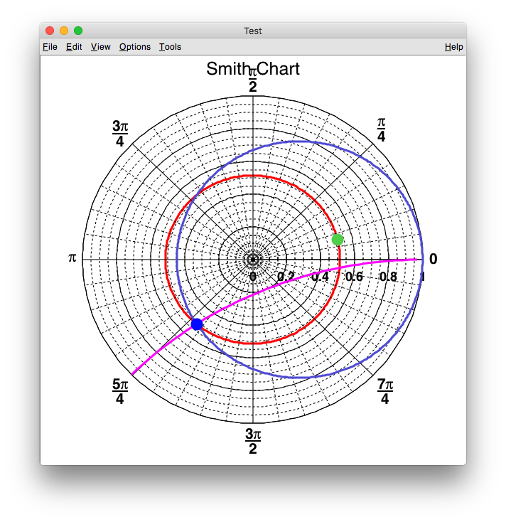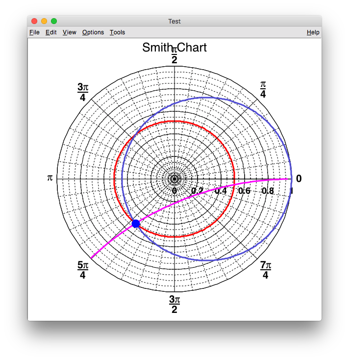
You can write the Smith chart with ROOT once you get Z(DUT), and therefore, the reflection coefficient. Note that the Smith chart is merely a polar plot of the reflection coefficient on a complex plane, limited within a radius of 1.0.
In the figure, the blue dot shows the reflection coeffcient of (-0.328107, -0.394757i), or (0.51395, -129.818 deg). The red circle shows the constant Abs(reflection coefficient) circle, or equivalently, the constant VSWR circle.
With a different length of the coaxial cable between your antenna and the measuring circuit, you will have your blue dot in other places, but they are always on the same red circle, ignoring the cable loss.
// file name = mytest45.cc
{
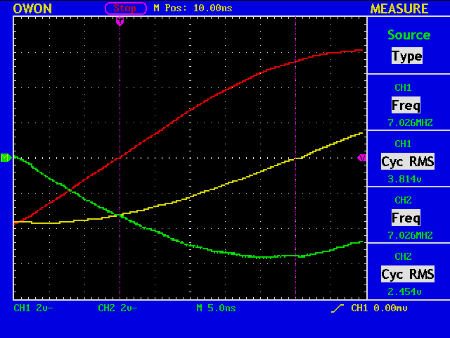
ifstream finput("owondata2.txt");
Int_t iskip=8;
std::string s;
for(int i=0;i<iskip;i++) {
getline(finput, s);
}
const Int_t icount_max=8192;
Int_t icount=0;
Double_t dummy, data1[icount_max], data2[icount_max], data3[icount_max];
while(icount < icount_max) {
finput >> data1[icount] >> dummy >> data2[icount] >> data3[icount];
if(finput.eof()) break;
icount++;
}
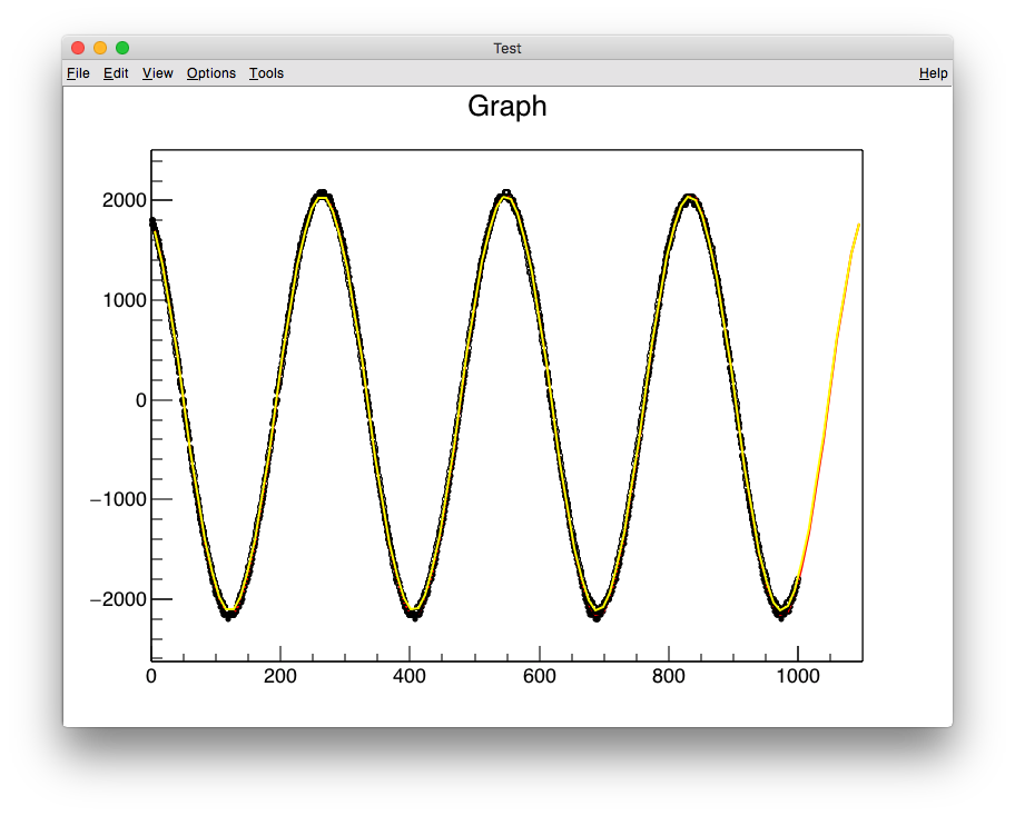
TCanvas *c1 = new TCanvas("c1","Test",0,0,800,600);
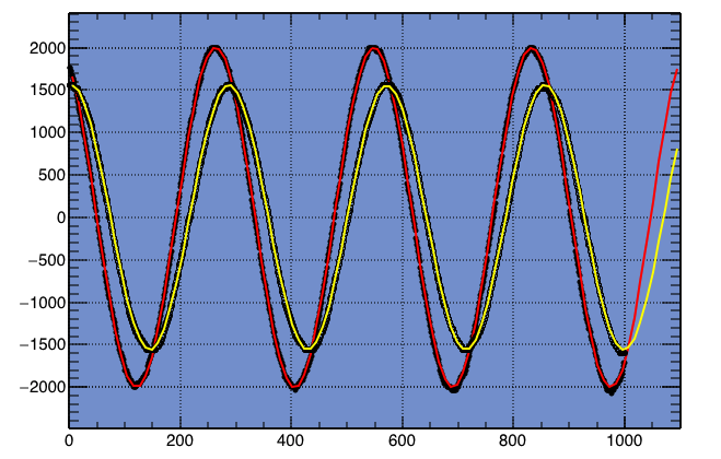
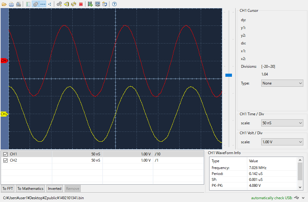
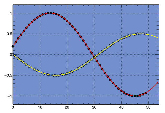
TGraph *g = new TGraph(icount, data1, data2);
g->SetMarkerStyle( 20 );
g->SetMarkerSize( 0.5 );
g->Draw("AP");
TF1 *f1 = new TF1("f1", "[0]*sin([1]*x+[2])-[3]");
f1->SetParameter(0, 2000.0);
f1->SetParameter(1, 0.022);
f1->SetParameter(2, 0.0);
f1->SetParameter(3, 0.0);
f1->SetLineColor(kRed);
g->Fit(f1);
TGraph *h = new TGraph(icount, data1, data3);
h->SetMarkerStyle( 24 );
h->SetMarkerSize( 0.5 );
h->Draw("P");
TF1 *f2 = new TF1("f2", "[0]*sin([1]*x+[2])-[3]");
f2->SetParameter(0, 2000.0);
f2->SetParameter(1, 0.022);
f2->SetParameter(2, 0.0);
f2->SetParameter(3, 0.0);
f2->SetLineColor(kYellow);
h->Fit(f2);
double amp, phase;
amp = f2->GetParameter(0) / f1->GetParameter(0);
phase = f2->GetParameter(2) - f1->GetParameter(2);
std::cout << "amp=" << amp << ", phase=" << phase << std::endl;
TComplex v1, v2, v3, Z, z50;
v1 = TComplex(1.0, 0.0);
v2 = TComplex( amp*TMath::Cos(phase), amp*TMath::Sin(phase) );
v3 = 2.0*v1 - v2;
z = v2/v3;
z50 = 50.0*z;
std::cout << "v1=" << v1 << ", v2=" << v2 << ", v3=" << v3 << ", z=" << z << ", z50=" << z50 << std::endl;
TComplex gg;
double gg_rho, gg_theta, vswr;
gg = (z-1.0)/(z+1.0);
vswr = (1.0+TComplex::Abs(gg)) / (1.0-TComplex::Abs(gg));
std::cout << "gg=" << gg << ", abs=" << TComplex::Abs(gg) << std::endl;
std::cout << "gg=" << gg.Rho() << ", " << gg.Theta()*360.0/(2.0*TMath::Pi()) << std::endl;
std::cout << "vswr=" << vswr << std::endl;
TCanvas * CPol = new TCanvas("CPol", "Test", 900, 0, 600, 600);
const Int_t ncircle = 360;
Double_t radius[ncircle];
Double_t theta [ncircle];
for (int i=0; i<ncircle; i++) {
radius[i] = gg.Rho();
theta [i] = TMath::Pi()*2.0*(double)i/(double)(ncircle-1);
}
Double_t radius_r[ncircle];
Double_t theta_r [ncircle];
Double_t r_center = z.Re() / (z.Re()+1.0);
Double_t r_radius = 1.0 / (z.Re()+1.0);
for (int i=0; i<ncircle; i++) {
Double_t th = TMath::Pi()*2.0*(double)i/(double)(ncircle-1);
Double_t re = r_center + r_radius*TMath::Cos(th);
Double_t im = r_radius*TMath::Sin(th);
TComplex ww = TComplex(re, im);
radius_r[i] = ww.Rho ();
theta_r [i] = ww.Theta();
}
Double_t radius_x[ncircle];
Double_t theta_x [ncircle];
TComplex x_center = TComplex(1.0, 1.0/z.Im());
Double_t x_radius = 1.0/ z.Im();
for (int i=0; i<ncircle; i++) {
Double_t th = TMath::Pi()*2.0*(double)i/(double)(ncircle-1);
Double_t re = x_center.Re() + x_radius*TMath::Cos(th);
Double_t im = x_center.Im() + x_radius*TMath::Sin(th);
TComplex ww = TComplex(re, im);
radius_x[i] = ww.Rho ();
theta_x [i] = ww.Theta();
}
TGraphPolar * grP1 = new TGraphPolar(ncircle, theta, radius);
grP1->SetTitle("Smith Chart");
grP1->SetMarkerStyle(20);
grP1->SetMarkerSize(2.0);
grP1->SetMarkerColor(4);
grP1->SetLineColor(2);
grP1->SetLineWidth(3);
grP1->Draw("C");
CPol->Update();
grP1->GetPolargram()->SetToRadian();
grP1->GetPolargram()->SetRangeRadial(0,1);
TGraphPolar * grP2 = new TGraphPolar(ncircle, theta_r, radius_r);
grP2->SetMarkerStyle(20);
grP2->SetMarkerSize(2.0);
grP2->SetMarkerColor(4);
grP2->SetLineColor(9);
grP2->SetLineWidth(3);
grP2->Draw("C");
TGraphPolar * grP3 = new TGraphPolar(ncircle, theta_x, radius_x);
grP3->SetMarkerStyle(20);
grP3->SetMarkerSize(2.0);
grP3->SetMarkerColor(4);
grP3->SetLineColor(6);
grP3->SetLineWidth(3);
grP3->Draw("C");
TMarker *m0 = new TMarker(gg.Re(), gg.Im(), 20);
m0->SetMarkerSize(2.0);
m0->SetMarkerColor(4);
m0->Draw();
}
% root mytest45.cc
amp=0.778415, phase=-0.53185
v1=(1,0i), v2=(0.670893,-0.394757i), v3=(1.32911,0.394757i), z=(0.382788,-0.410701i), z50=(19.1394,-20.535i)
gg=(-0.329107,-0.394757i), abs=0.51395
gg=0.51395, -129.818
vswr=3.1148