Tag: Antenna

I removed the elements for 21MHz and 28MHz and used them as a single element. Since 15m+10m=25m, it should be resonant somewhere around 12MHz.

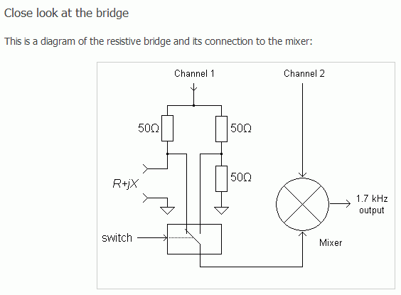
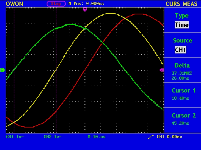
At 7026kHz, the measurement using a bridge tells that V1=2.569 V, V2=0.869 V, and V2delay=24.20 nS, which means Z=2.629+j8.624 ohm, and SWR=19.6.

Considering the cable length of 20m, Zant=14.861-j108.951 ohm.

At 10110kHz, V1=3.083 V, V2=5.222 V, and V2delay=4.40 nS, which gives Z=54.274+j131.008 ohm, and SWR=8.20, and Zant=29.910+j95.210 ohm.

At 14010kHz, V1=2.599 V, V2=2.495 V, V2delay=-9.40 nS, which gives Z=8.131-j30.425 ohm, and SWR=8.47, and Zant=5.906-j1.093 ohm.

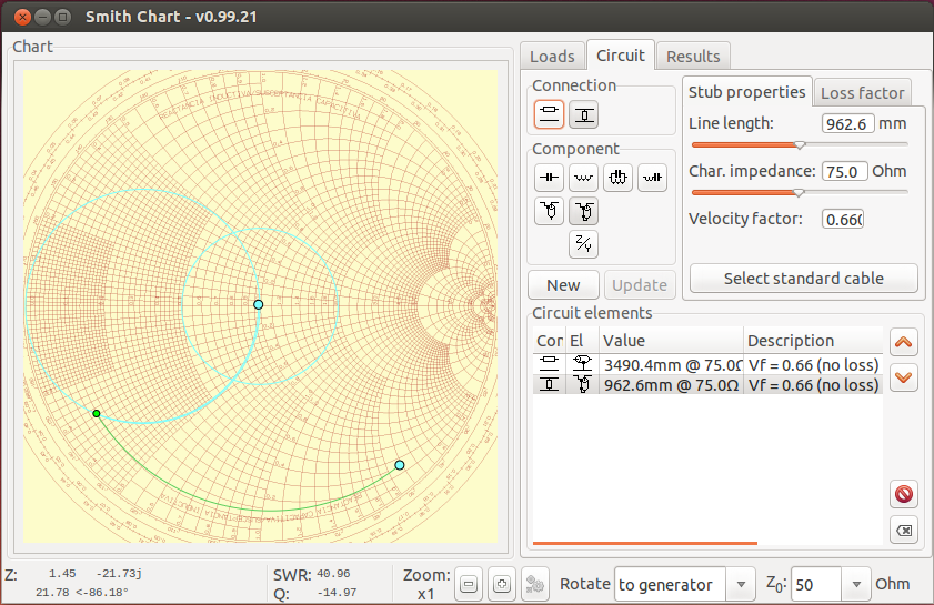
For stub matching at 7026kHz, we need a 3490.4 mm cable and a 962.6mm short-circuited cable both 75 ohm to obtain Z=49.383+j0.774 ohm.

The above figure is from “AA-30/AA-54 Analyzers, How it works?”
http://www.rigexpert.com/index?s=aa54&f=inside

The bridge circuit is the same as the one shown in my previous post:
Directional Bridge (November 5, 2013).

Instead of down-converting the signals to be A/D connverted, I am simply using an oscilloscope to directly observe the amplitude and the phase of the signals.

The red (CH1) and yellow (CH2) traces correspond to the signals obtained from the bridge, and the green trace to CH1 – CH2.

From “Network Analyzer Basics”, Agilent Technologies, slide 126.

This is my directional bridge for measuring antenna impedance.

Two more nice slides from the same document.

Now let’s try stub matching. The length of 75 ohm coax cables required is 531.4mm for d1 and 1182.4mm (with open end) for d2.

This is to calibrate the measurement system using a dummy load.

This is my antenna with stub matching. Looks nice. Almost as good as a dummy load.

gnuplot> load "gnuplot1.txt"
Freq [MHz]=28.001
V1=2.122
V2=2.362
Cursor 1=0.0
Cursor 2=0.0

vratio=1.11310084825636
phase1 [deg]=0.0
phase2 [deg]=0.0

abs(gamma)=0.113100848256362
swr=1.25504782146653
cz=62.7523910733263

Without stub matching, the VSWR was 2.61, so there is definitely much improvement.

The measured impedance of cz={89.9733735327047, -55.8789510601876} is traslated to the feed point impedance by using a Smith Chart.

Assuming the cable length of 20m, Zant={19.398, -8.999}.

If the cable length is 20m+10cm, then Zant={20.170, -12.965}, and if it is 20m-10cm, then Zant={18.919, -5.117}.

Parameters for stub match with 75 ohm coax cables are: 531.4mm and 1182.4mm (with open end).

First, calibration of the measurement system using a dummy load. There is almost no reflected wave (in green).

This is at 28.001MHz.

gnuplot> load "gnuplot1.txt"
Freq [MHz]=28.001
V1=2.518
V2=3.539
Cursor 1=-1e-009
Cursor 2=0.0

vratio=1.4054805401112
phase1 [deg]=-10.08036
phase2 [deg]=0.0

abs(gamma)=0.455858107934516
swr=2.67551190078067
cz={89.9733735327047, -55.8789510601876}

The VSWR is 2.67, and this figure matches well with the read out from a Power Meter.

The forward power is 15 W and the reflected power is 3 W. The normalized reflect voltage is sqrt(3/15)=0.4472, thus the VSWR=(1+0.4472)/(1-0.4472)=2.61.

Mostly on 40m band, mode CW, and ANT is dipole, POW 20-30W.

Now, let’s think of a case, for example, in which Z=10+jX.

This time Z can be anywhere on the r=0.2 circle (outer brown circle) and you can see from the figure that Z is again most close to the origin (red dot) when X=0.

See that the two brown circles (outer and inner ones) are mutually tangent to each other, the point of the contact being at X=0.

In general, the feed point impedance of an antenna is Z=R+jX, where R could be either greater than or less than 50 ohm.

First, let’s think of a case, for example, in which Z=100+jX. Now Z can be anywhere on the r=2 circle (blue on the right) and it is obvious that Z is most close to the origin (red dot) when X=0.

This can also be confirmed by looking at the two blue circles which are mutually tangent to each other, the point of the contact being at X=0.

The same can be said for any R > 50, which you can see immediately from the figure if you imagine two such blue circles.

(picture from [1], but the color added by the author.)

So we would like to know if an antenna in resonance gives the minimum VSWR, under the assumption that only the imaginary part of the feed point impedance varies when when we change the element length.

Let’s assume for the moment that the system impedance Z0 is 50 ohm, and if we further assume that the feed point impedance is given by "Z=50+j*X", then Z is always on the r=1 circle (green), and in this case obviously Z is most close to the origin (red dot) when X=0.

Actually in this particular case, Z becomes exactly 50 ohm when X=0, and coincides with Z0, thus the complex reflection coefficient gamma is 0, which means rho is also 0 and VSWR=1.

[1] http://www.arrl.org/files/file/Antenna%20Book%20Supplemental%20Files/22nd%20Edition/Smith%20Chart%20Supplement%20-%20Corrected%20Jan%202012.pdf