Month: May 2013

Data sets in R are most often stored in data frames. A data frame is a two dimensional data structure, with each row representing a case and each column reresenting a variable. You can generate a data frame, for example, from vectors as in the following way, where each vector represents a column.

> name    <- c("Alpha", "Bravo", "Charlie", "Delta")
> weight  <- c(31.0, 47.2, 69.5, 99.8)
> price   <- c(9.2, 13.7, 21.4, 38.5)
> example <- data.frame(name, weight, price)
> example
     name weight price
1   Alpha   31.0   9.2
2   Bravo   47.2  13.7
3 Charlie   69.5  21.4
4   Delta   99.8  38.5

Once you have a data frame, it is a relatively simple task to analyze the data and to draw graphs of various types.

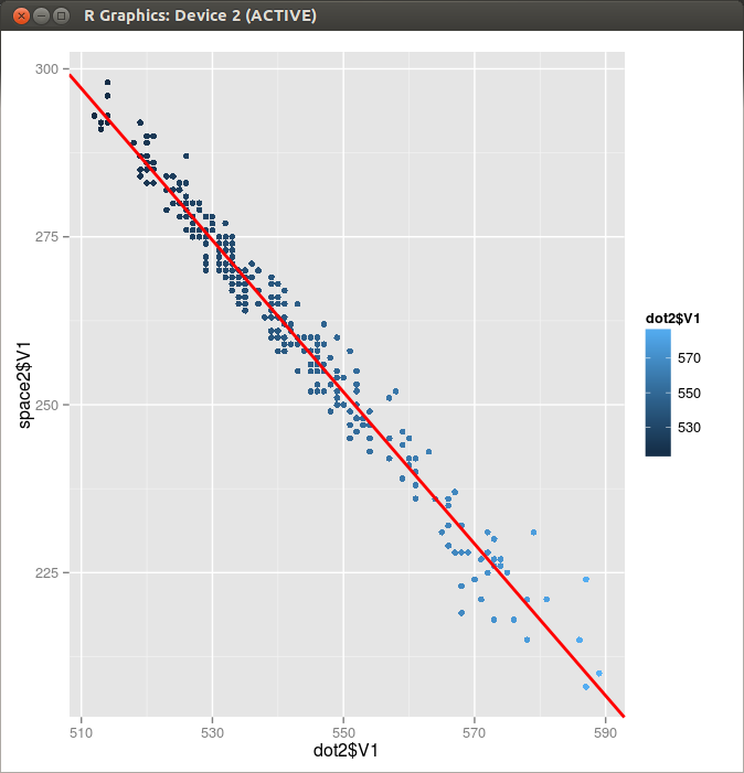
> graph <- ggplot(example, aes(x=weight, y=price))
> graph + geom_point() + stat_smooth(method=lm)

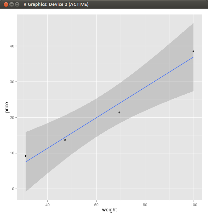
Figure 1. Scatter Plot and a Linear Regression Line

        letter_space      11688          0
                 dot        510          0
       element_space        265          0
                 dot        533          1
       element_space        341          0
                 dot        511          2
       element_space        333          0
                 dot        499          3
        letter_space       1451          0
                 dot        541          0
       element_space        530          0
                dash       1647          0
       element_space        281          0
                 dot        505          1
        letter_space       2539          0
           (853 more lines deleted..)

Here is a first part of the output from “myprog” which reads a file containing Morse code that starts with “HR HR” by JO1FYC.
[1] http://homepage2.nifty.com/jo1fyc/sound/20051010_nikki-32.mp3

This is a text file and readily loaded into R by using read.table().

> mydata <-read.table("20051010_nikki-32_8kHz.aaa", header=FALSE)
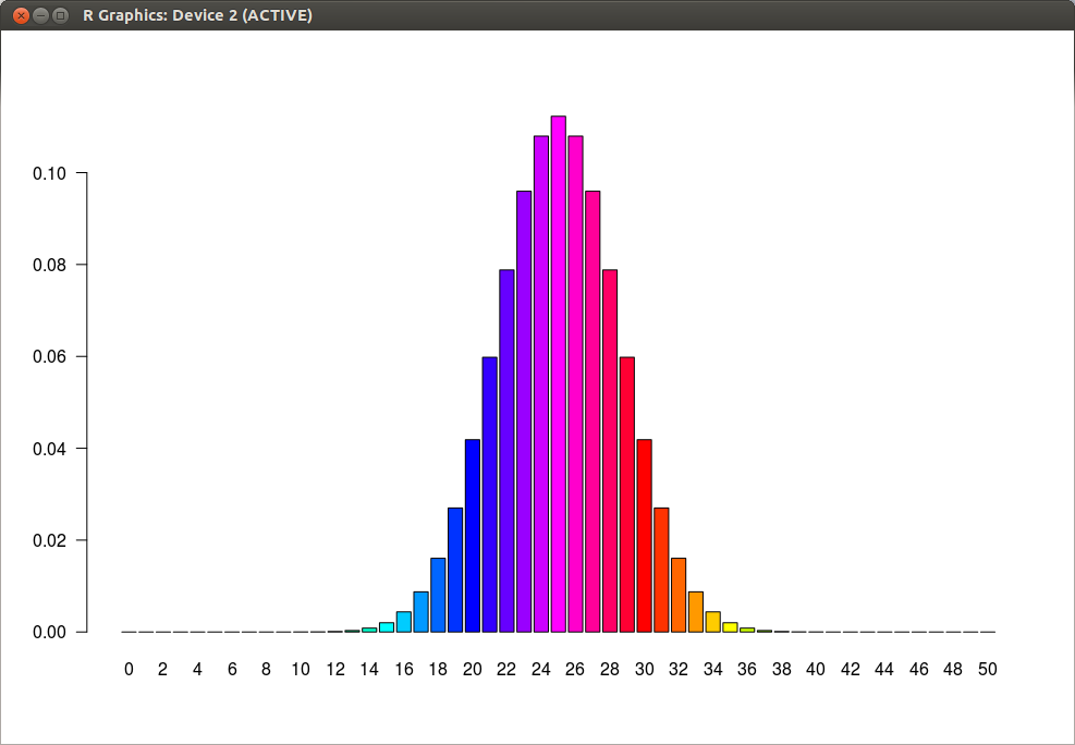
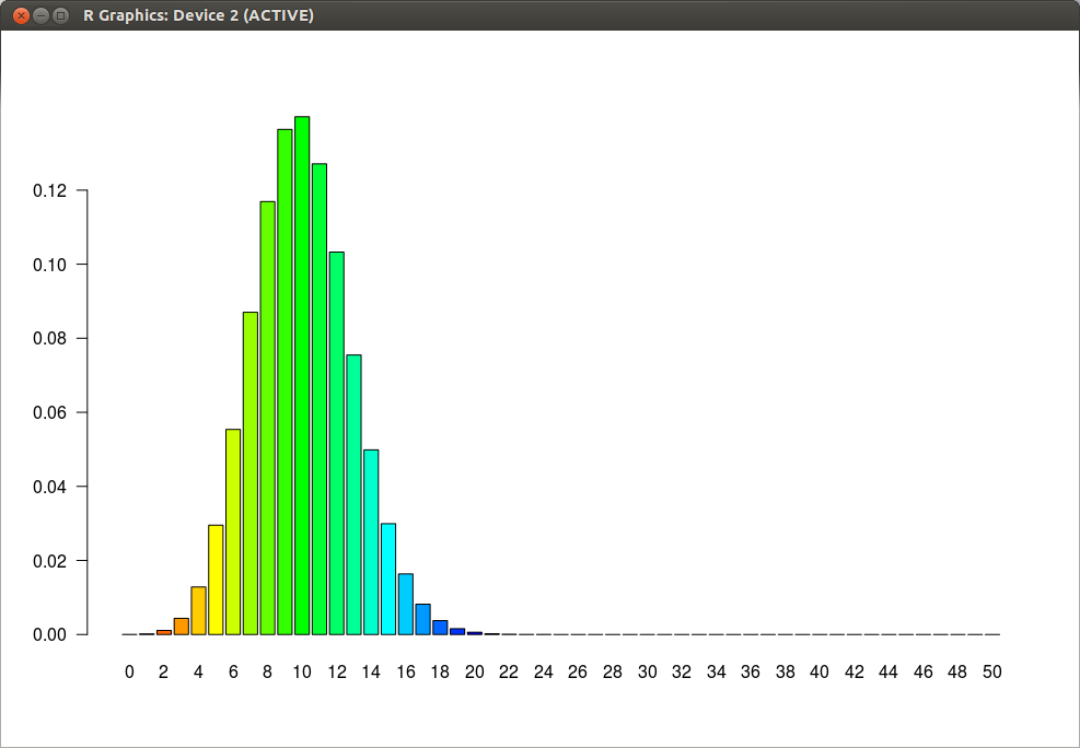
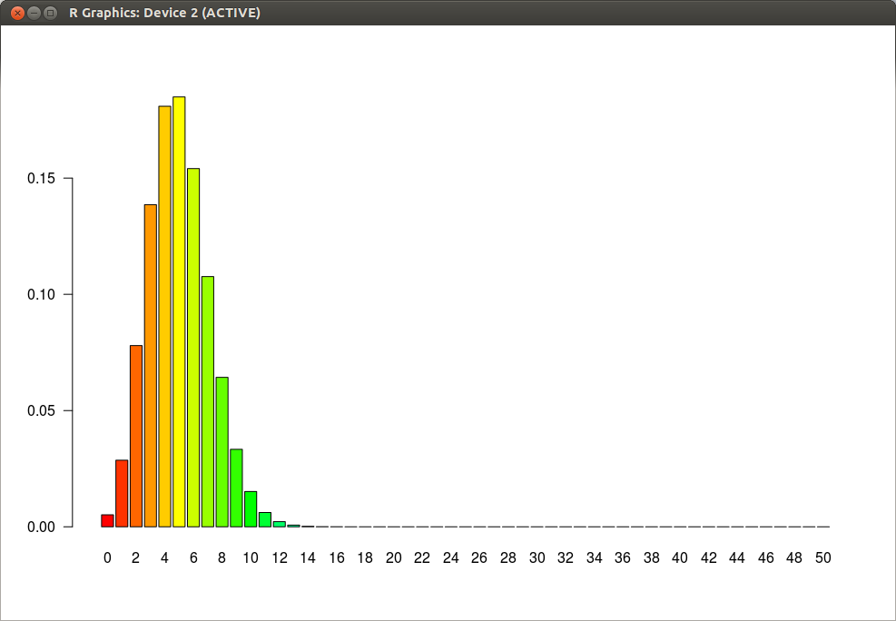
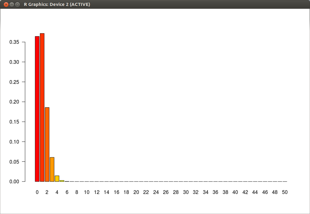
> ggplot(mydata, aes(x=V1, fill=V1)) + geom_histogram()

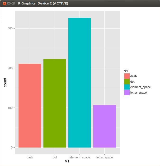
Figure 2. Histogram

It seems that the duration of dot cycle is almost constant except for the last few seconds. So I extracted a “nice part” of the dot and space duration data from the originals by discarding the first ten and the last sixty-two points, and tried to find the line of best fit by applying a linear model.

Figure 1. Dot and Space pair in a Single Dot Cycle

> dot2   <- read.table("BK2.dot"  ,header=FALSE)
> space2 <- read.table("BK2.space",header=FALSE)
> res=lm(space2$V1~dot2$V1)
> res

Call:
lm(formula = space2$V1 ~ dot2$V1)

Coefficients:
(Intercept)      dot2$V1
     873.38        -1.13

> p <- qplot(dot2$V1,space2$V1,color=dot2$V1)+geom_point(shape=23,size=1)
> p+ geom_abline(intercept=873.38, slope=-1.13, colour="red", size=1)

Draw the same graphs with the library ggplot2.

Figure 1. Dot Length

Figure 2. Space Length

Figure 3. Duration of Dot Cycle

JO1FYC [1] offers some mp3 files of his Morse music in his blog [2], and I was tempted to anylize the latest one [3], dated May 6, 2013. Since the file contains a series of consecutive dots with a bug key, it might give some good parameters for a physical model of such keys.
[1] http://homepage2.nifty.com/jo1fyc/index.htm
[2] http://homepage2.nifty.com/jo1fyc/cw_nikki.htm
[3] http://homepage2.nifty.com/jo1fyc/sound/BK-100_DOT_20130506.mp3

Figure 1. Dot and Space Length

The dots continue more than 30 sec, and you can count 362 dots. The lengh of each dot is incresing slowly for the most of the time, and for the last few seconds it increases rather rapidly.

Figure 2. Dot Length

Figure 3. Space Length

Figure 4. Duration of Dot Cycle

The figures are obtained by the following commands.

% mplayer -quiet -vo null -vc dummy -af volume=0,resample=8000
          -ao pcm:waveheader:file="BK-100_DOT_20130506_8kHz.wav"
          "BK-100_DOT_20130506.mp3"
% myprog BK-100_DOT_20130506_8kHz.wav > BK.txt
% awk '{if($1=="dot" || $1=="dash") print $2}' BK.txt > BK.dot
% awk '{if($1=="element_space")     print $2}' BK.txt > BK.space

% gnuplot
gnuplot> plot "BK.dot" with line, "BK.space" with line

% R
> dot   <-read.table("BK.dot",   header=FALSE)
> space <-read.table("BK.space", header=FALSE)
> added=dot$V1 + space$V1
> plot(dot$V1)
> plot(space$V1)
> plot(added)