
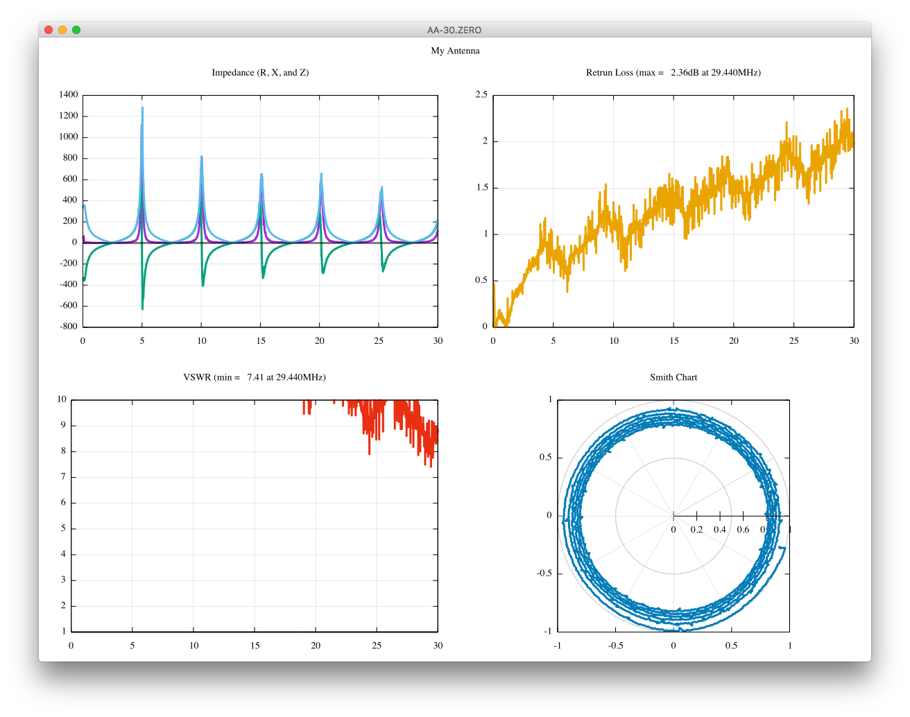
I am using a 20m coaxial cable (5D-2V) and its far end is left open during the measurement.
The Smith Chart tells you everything, but it is easier to see its amplitude and phase separately.
First, the amplitude in dB.
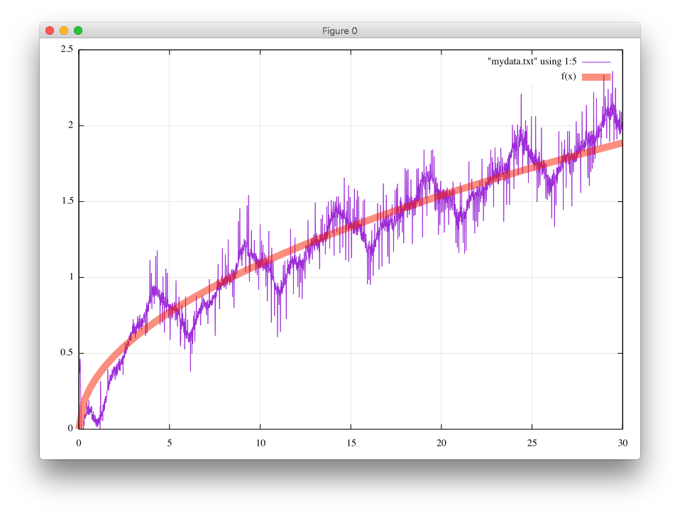
% gnuplot
gnuplot> f(x)=a*sqrt(x)
gnuplot> fit f(x) "mydata.txt" using 1:5 via a
iter      chisq       delta/lim  lambda   a
   0 9.0593050625e+02   0.00e+00  8.02e-01    2.070472e-01
   1 5.4539304323e+01  -1.56e+06  8.02e-02    3.445278e-01
   2 5.4539209850e+01  -1.73e-01  8.02e-03    3.445736e-01
iter      chisq       delta/lim  lambda   a

After 2 iterations the fit converged.
final sum of squares of residuals : 54.5392
rel. change during last iteration : -1.7322e-06

degrees of freedom    (FIT_NDF)                        : 3000
rms of residuals      (FIT_STDFIT) = sqrt(WSSR/ndf)    : 0.134832
variance of residuals (reduced chisquare) = WSSR/ndf   : 0.0181797

Final set of parameters            Asymptotic Standard Error
=======================            ==========================
a               = 0.344574         +/- 0.0006355    (0.1844%)
gnuplot> print a*sqrt(30)
1.88730727013936
The loss of 1.887[dB] at 30MHz agrees well with its nominal value of 0.44dB/10m, or 1.76dB/40m.
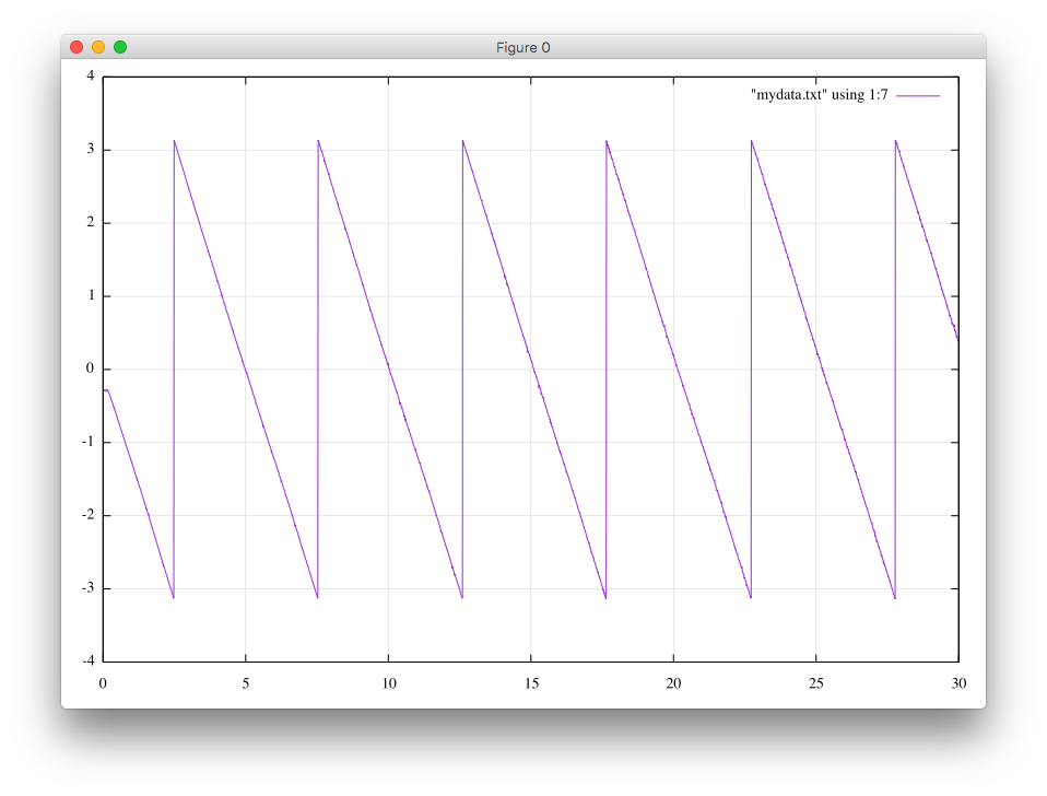
Next, the phase in radian.
 .
.
Let’s see at which frequencies the phase changes from -pi to +pi.
 2.48, 1.3514, -0.299513, 1.3842, 0.469624, 36.9999, -3.1296, 0.947368
 2.49, 1.39451, 0.083306, 1.397, 0.484627, 35.8549, 3.13826, 0.945733

 7.53, 2.59869, -0.289392, 2.61476, 0.903662, 19.2411, -3.12999, 0.901191
 7.54, 2.45728, 0.08333, 2.4587, 0.854434, 20.3477, 3.13825, 0.906313

 12.6, 3.4673, -0.351551, 3.48508, 1.20654, 14.4212, -3.12746, 0.870308
 12.61, 3.43064, 0.097069, 3.43201, 1.1938, 14.5746, 3.13769, 0.871586
...
 27.77, 5.43172, -0.091826, 5.43249, 1.89464, 9.20522, -3.13788, 0.804022
 27.78, 5.31208, 0.100171, 5.31302, 1.85259, 9.41255, 3.13754, 0.807924
The period is (27.77MHz-2.48MHz)/5cyles, which is 5.06MHz/cycle.
The electrical length of the cable is thus (300m*MHz/5.06MHz)/2=29.64m.
Assuming the velocity factor of 66%, the physical length is known to be 19.56m.