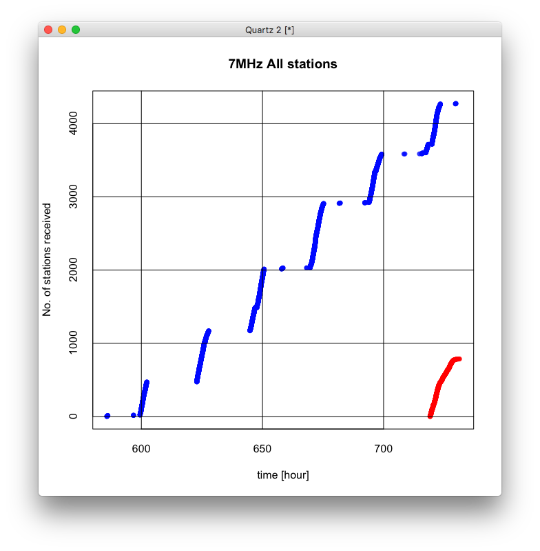
ADIF data for the last week.
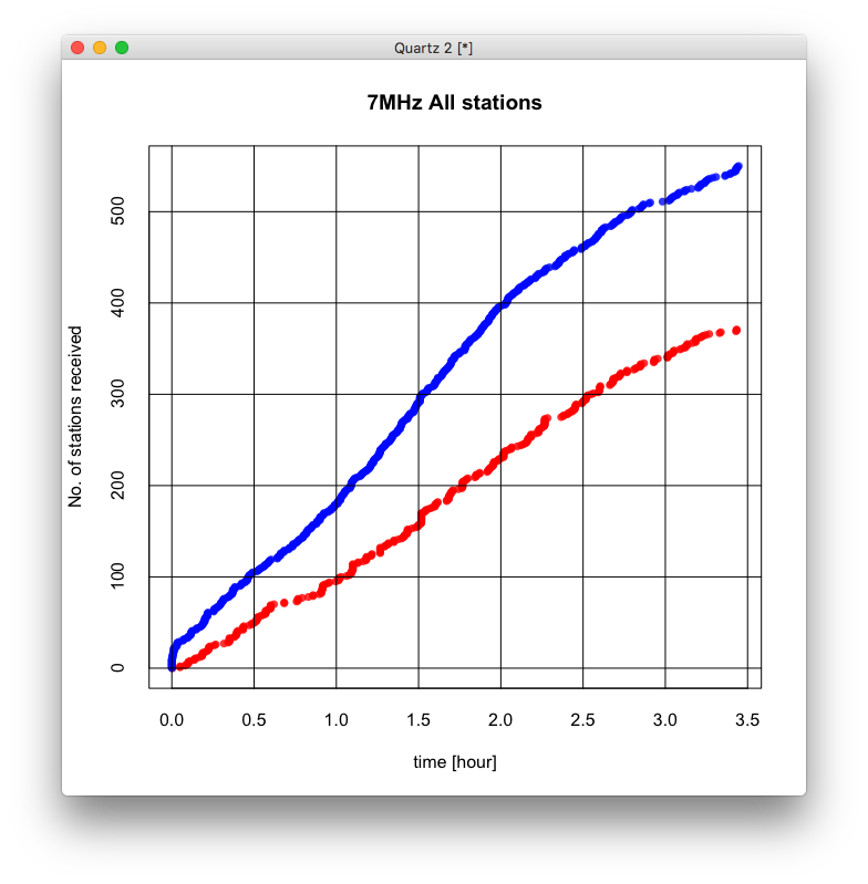
Just for the last several hours.
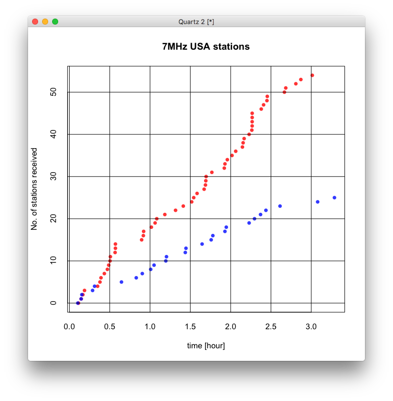
Only the USA stations.

Ham Radio Blog
ADIF data for the last week.
Just for the last several hours.
Only the USA stations.
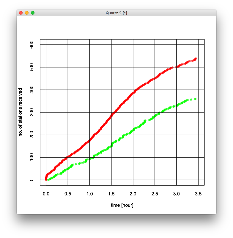
Not QSO rates, but reporting rates. The graph is for all stations.
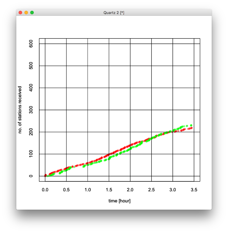
This is for Non-JA stations.
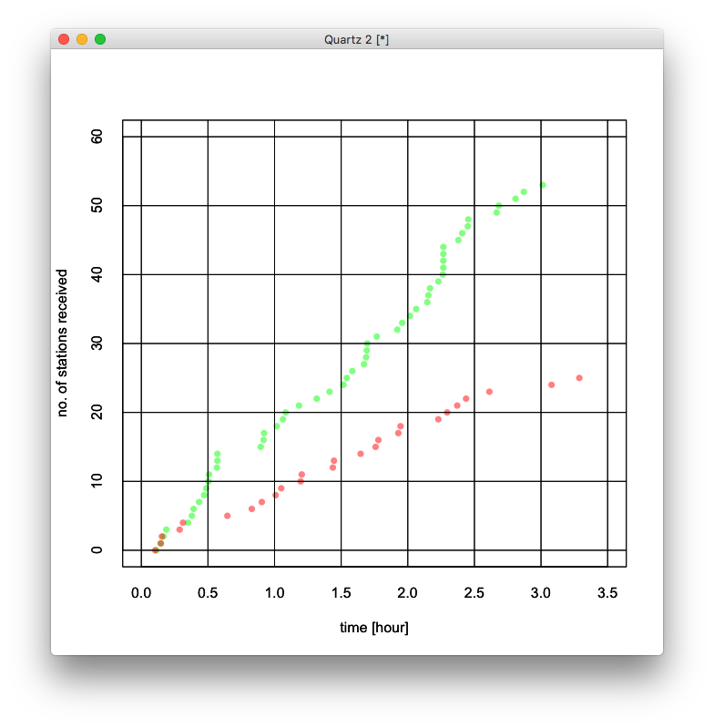
This is for USA stations only.
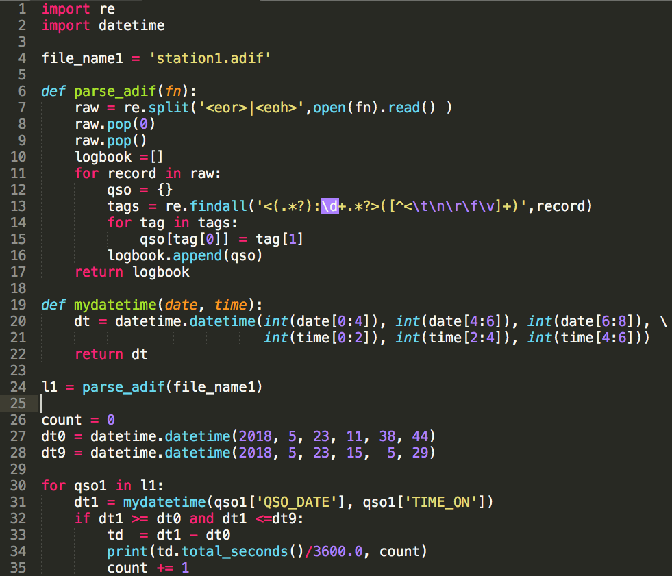
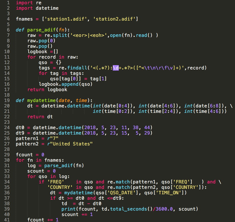
import re
import datetime

file_name1 = 'station1.adif'

def parse_adif(fn):
    raw = re.split('<eor>|<eoh>',open(fn).read() )
    raw.pop(0)
    raw.pop()
    logbook =[]
    for record in raw:
        qso = {}
        tags = re.findall('<(.*?):\d+.*?>([^<\t\n\r\f\v]+)',record)
        for tag in tags:
            qso[tag[0]] = tag[1]
        logbook.append(qso)
    return logbook

def mydatetime(date, time):
    dt = datetime.datetime(int(date[0:4]), int(date[4:6]), int(date[6:8]), \
                           int(time[0:2]), int(time[2:4]), int(time[4:6]))
    return dt

l1 = parse_adif(file_name1)

count = 0
dt0 = datetime.datetime(2018, 5, 23, 11, 38, 44)
dt9 = datetime.datetime(2018, 5, 23, 15,  5, 29)

for qso1 in l1:
    dt1 = mydatetime(qso1['QSO_DATE'], qso1['TIME_ON'])
    if dt1 >= dt0 and dt1 <=dt9:
        td  = dt1 - dt0
        print(td.total_seconds()/3600.0, count)
        count += 1
% cat stationXYZ.adif | grep FREQ:8\>7\. | grep PSKREP | grep -v Japan > station1.adif
% python3 adif_parse.py > data1.csv
% R
> data1=read.csv("data1.csv", header=F, sep="")
> data2=read.csv("data2.csv", header=F, sep="")
> plot(data1$V1, data1$V2, xlab="time [hour]", ylab="no. of stations received", pch=16, col="#00ff0080", tck=1, xlim=c(0.0, 3.5), ylim=c(0,600))
> par(new=T)
> plot(data2$V1, data2$V2, xlab="time [hour]", ylab="no. of stations received", pch=16, col="#ff000080", tck=1, xlim=c(0.0, 3.5), ylim=c(0,600))