Month: July 2013

I have some 2SK192As in my junk box, and need to make a device model for LTspice.

The parameters (beta, vto, etc.) are quite tentative and will be adjusted after measuring the devices at hand.

Note: Idss Clasiffication Y:3.0-7.0, GR:6.0-14.0, BL:12.0-24.0.

“I1” is the current output (IOUT) of AD9834.

Soft66LC4, a direct conversion receiver, includes a DDS device, AD9834, for LO.

The figure shows its IOUT (pin 20) signal. The 3.513MHz signal from the device is doubled on the board to get 7.026MHz set by the control software.

The element length is trimmed by 2cm for three times.

The coax cable for a 17m band dipole is terminated with a 100 ohm resistor at far end, temporarily removing the antenna elements.

(%i) V1:1.0+%i*0.0;
(%i) t:2.0*3.1416*(-22.0e-9/(1/1.91e6));
(%i) s:2.175/2.682;
(%i) V2:s*(cos(t)+%i*sin(t));
(%i) Vr:2*V1-V2;
(%i) z:50.0*V2/Vr;
(%i) realpart(z);
(%o) 29.74885022942517
(%i) imagpart(z);
(%o) -13.86642130849026
(%i) abs(z);
(%o) 32.8218178941588
(%i) g:(z-50)/(z+50);
(%i) abs(g);
(%o) 0.30321141723506
(%i) SWR:(1+abs(g))/(1-abs(g));
(%o) 1.870311095029369

The impedance at the near end is therefore Z=29.7-i13.9 ohm.

With a 20m cable, the impedance at far end should be Z=93.4+i3.4 ohm, which sounds reasonable.

First, with a dummy load. This seems to be quite reasonable. Almost no reflection (green), and V1 (red) and V2 (yellow) are almost the same.

Then, my 17m band full-size dipole, which is far from satisfactory.

The voltage ratio V2/V1=0.9085/2.259=0.402, and the delay of V2 against V1 is 41.7deg (=360deg*6.40nS/55.2nS).

The magnitude of the reflection coefficient is 0.749, which corresponds to the VSWR of 6.98.

(%i) V1:1.0+%i*0.0;
(%i) t:2.0*3.1416*(-41.7/360.0);
(%i) V2:0.402*(cos(t)+%i*sin(t));
(%i) Vr:2*V1-V2;
(%i) z:50.0*V2/Vr;
(%i) realpart(z);
(%o) 7.407809291003613
(%i) imagpart(z);
(%o) -9.031478001791401
(%i) abs(z);
(%o) 11.68089180622445
(%i) g:(z-50)/(z+50);
(%i) abs(g);
(%o) 0.74920478622757
(%i) SWR:(1+abs(g))/(1-abs(g));
(%o) 6.974633845344225

The cable length is, if I remember correctly, around 20m, so the antenna impedance should be 17.8+i59.4 ohm, but this is not very likely from the simulation below.

The same 9m coax cable but with its far end terminated with 100ohm.

At 1910kHz (T=523.6nS) the delay of V2 (yellow) against V1 (red) is +19.00nS (=+13.1deg) and V2-V1 (green) +91nS (=+62.6deg), whereas V1=2.939V and V2=3.463V (V2/V1=1.18).

Theoretically, the magnitude of the reflection coefficient in this case is (ZL-Zs)/(ZL+Zs)=1/3, and its phase is 61.6deg (=2.0*360.0*(9/0.67)/(300/1.91)), which gives the relationship between the incident wave (=V1, red) and the reflected wave (=V2-V1, green).

From the figure, you can see that V2 (yellow) should be mag=1.19 and phase=14.1 deg, both in good agreement with the measurement.

gnuplot> set object 1 rectangle from screen 0,0 to screen 1,1 fillcolor rgb "#f0f0f0" behind
gnuplot> set size square
gnuplot> set xrange[-0.5:2.5]
gnuplot> set yrange[-1.5:1.5]
gnuplot> set zeroaxis
gnuplot> set parametric
gnuplot> plot [0:2*pi] 1+cos(t)/3,sin(t)/3 lw 2 lt -1
gnuplot> set arrow 1 from 0.0 to 1.0 lw 2 lt -1
gnuplot> set arrow 2 from 1,0 to 1+cos(1.07)/3,sin(1.07)/3 lw 2 lt 2
gnuplot> set arrow 3 from 0,0 to 1+cos(1.07)/3,sin(1.07)/3 lw 2 lt 6
gnuplot> set arrow 4 from 0.0 to 2,0 lw 1 lt -1
gnuplot> set arrow 5 from 1+cos(1.07)/3,sin(1.07)/3 to 2,0 lw 2 lt 3
gnuplot> replot

The same configuration, but at 18100kHz. The phase of the reflection coefficient in this case becomes 583.5deg, or 223.5deg by subtracting 360deg.

From the figure, it is expected that V2 (yellow) is mag=0.79 and phase=-16.8 deg.

From the measurement, we see that V2 (yellow)/V1 (red)=2.334/2.560=0.911 and the phase of V2 relative to V1 is -19.6deg.

The DUT is a 9m coax cable with open end.

The voltage V1 is shown in red, V2 in yellow, and V2-V1 in green.

Note that since the magnitude (=the absolute value) of the reflection coefficient is 1.0, the impedance Z=R+iX of the DUT is always pure imaginary, whatever the cable length is, and therefore the vectors V2 and Vr6 are always mutually orthogonal. In other words, the terminal point of the vector V2 is always on the circle, and the angle of V2 against V1 is half the angle of V2-V1 against V1.

You can see that the delay of V2 (yellow) against V1 (red) is 45nS, and the delay of V2-V1 (green) against V1 is 90nS, just twice the value as is expected. Since the period T is 524nS (f=1910kHz), these correspond to the angles of 30.9deg and 61.8deg, respectively.

> At 1910kHz (T=523.6nS). The delay is +43.00nS (+29.6deg), V1=3.094V and V2=5.256V both measured using CH1 (V2/V1=1.70).

(%i) t:(-29.6/360.0)*2.0*%pi; <- negative for delay
(%i) s:1.7/2;
(%i) Vs:1.0+%i*0.0;
(%i) V2:s*(cos(t)+%i*sin(t));
(%i) Vr:Vs-V2;
(%i) z:50.0*(V2/Vr);
(%i) float(realpart(z));
(%o) 3.390649793776409
(%i) float(imagpart(z));
(%o) -85.90869167405812

Therefore, the impedance of the DUT, a 9m coax cable with open end, is Z=3.39-85.91i.

By using the Smith Chart, we get Z=0.01-82.38i with a 9m coax cable.

> At 3526kHz (T=283.6nS). The delay is +44.80nS (+56.9deg), V1=2.641V and V2=2.694V both measured using CH1 (V2/V1=1.02).

(%i) t:(-56.9/360.0)*2.0*%pi; <- negative for delay
(%i) s:1.02/2;
(%i) float(realpart(z));
(%o) 1.309389036427464
(%i) float(imagpart(z));
(%o) -30.38338285043538

The Smith Chart shows that Z=0.00-31.61i.

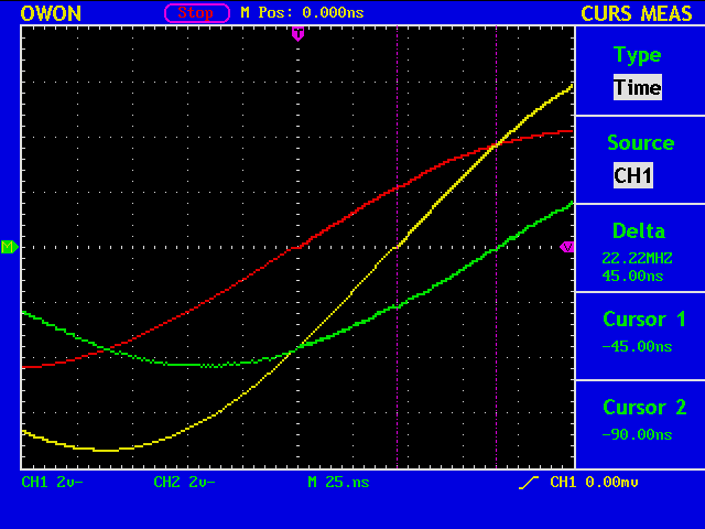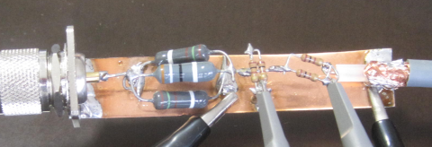
A coaxial cable (5D-2V) with length approx. 9m is used with its far end open.

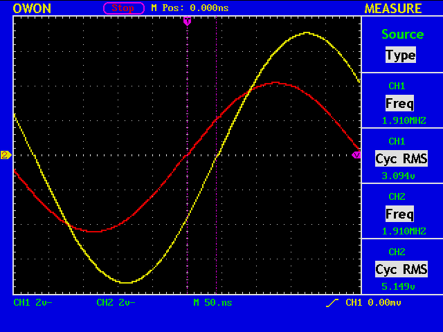
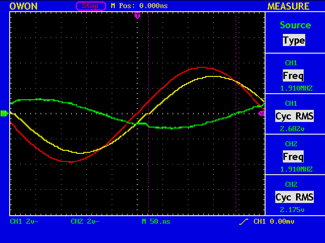
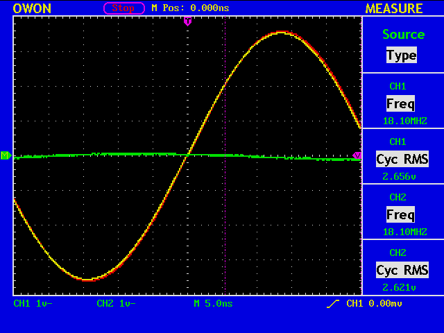
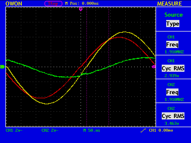
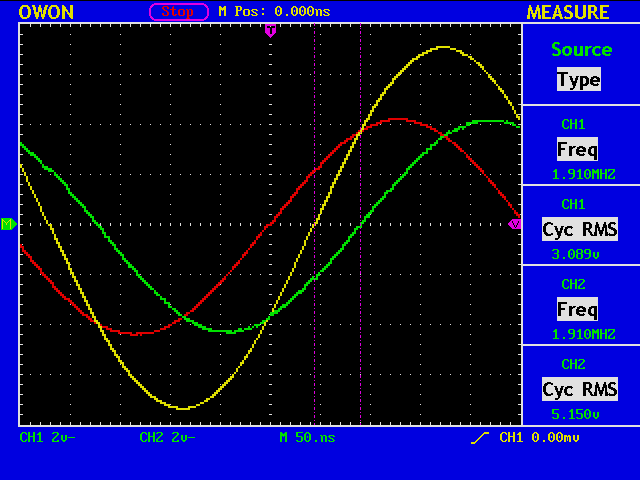
At 1910kHz (T=523.6nS). The delay is +43.00nS (+29.6deg), V1=3.094V and V2=5.256V both measured using CH1 (V2/V1=1.70).

Assuming the cable length is exactly 9m and with no cable loss (actually , the loss for 5D-2V is 26dB/km@10MHz.), the expectd delay should be:

(%i) t:2.0*360.0*(9.0/(300.0*0.67/1.91));
(%o) 61.57611940298507
(%i) tt:2.0*3.1416*(t/360.0);
(%o) 1.074708537313433
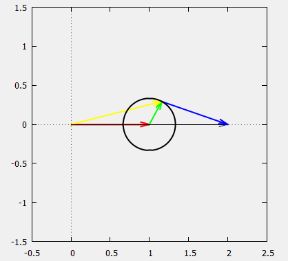
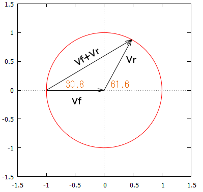
(%i) Vf:1.0+%i*0.0;
(%o) 1.0
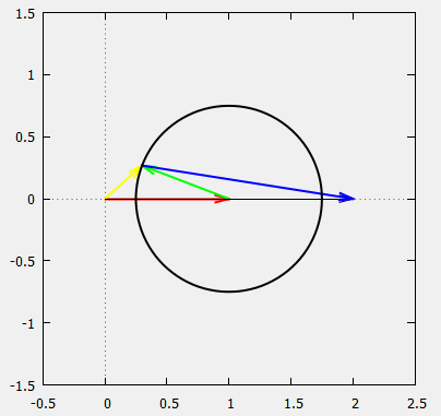
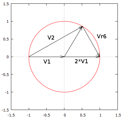
(%i) Vr:cos(tt)+%i*sin(tt);
(%o) 0.87945145487724*%i+0.47598859073964
(%i) abs(Vf+Vr);
(%o) 1.718131887102755
(%i) atan(imagpart(Vf+Vr)/realpart(Vf+Vr))/(2.0*3.1416)*360.0;
(%o) 30.78805970149254

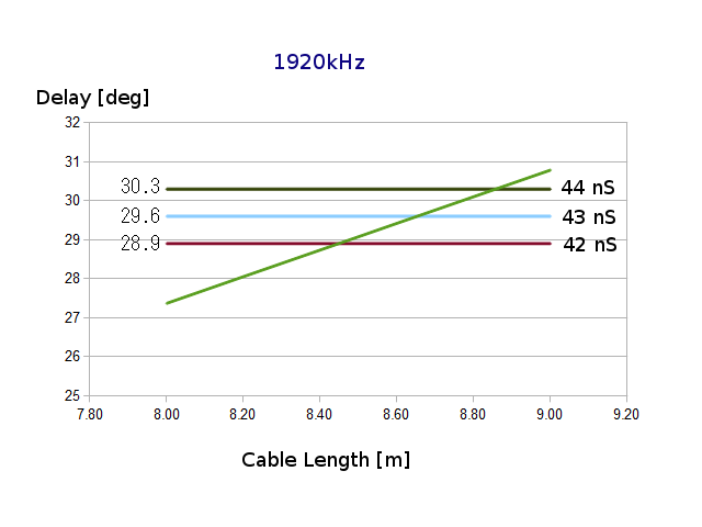
The delay is measured to be 43 [nS] at 1910kHz, but it could be anywhere between, say, 42[nS] and 44nS. In that case, the cable length could be somewhere between 8.45m and 8.85m.

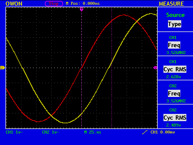
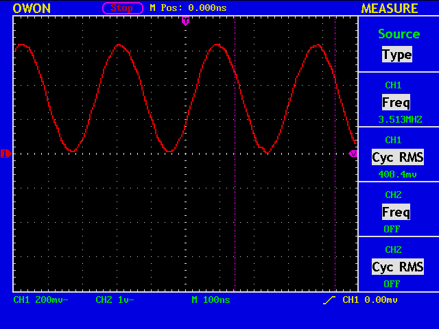
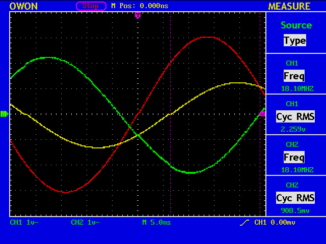
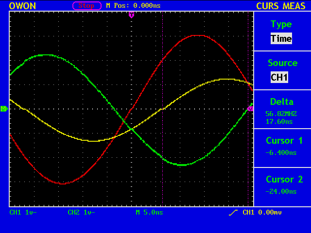
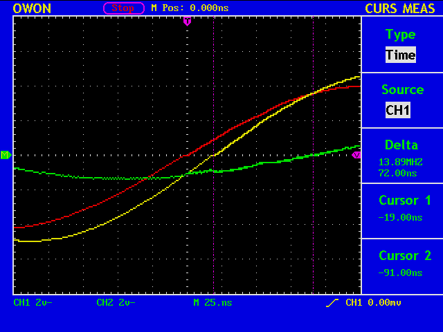
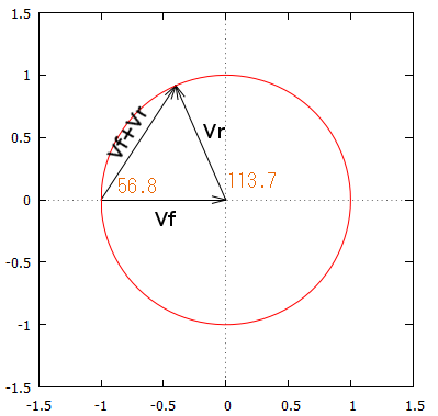
At 3526kHz (T=283.6nS). The delay is +44.80nS (+56.9deg), V1=2.641V and V2=2.694V both measured using CH1 (V2/V1=1.02).

(%i) t:2.0*360.0*(9.0/(300.0*0.67/3.526));
(%o) 113.6740298507463 <-phase rotation in deg
(%i) tt:2.0*3.1416*(t/360.0);
(%o) 1.983990734328358 <-phase rotation in rad
(%i) Vf:1.0+%i*0.0;
(%o) 1.0
(%i) Vr:cos(tt)+%i*sin(tt);
(%o) 0.91584282508565*%i-0.40153694691664
(%i) abs(Vf+Vr);
(%o) 1.094041181202386
(%i) atan(imagpart(Vf+Vr)/realpart(Vf+Vr))/(2.0*3.1416)*360.0;
(%o) 56.83701492537313

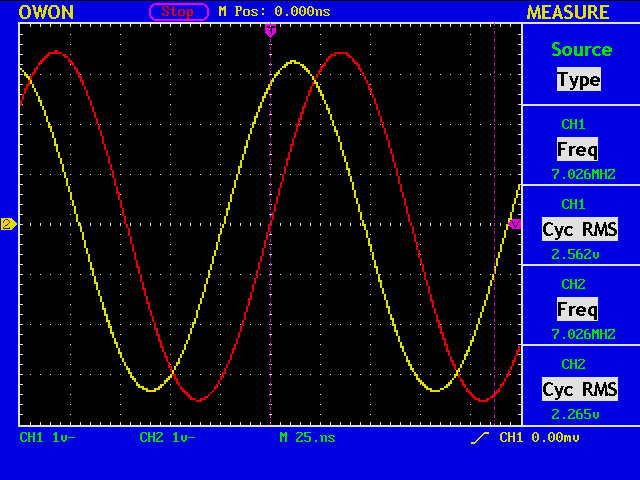
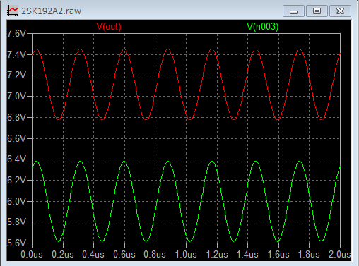
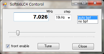
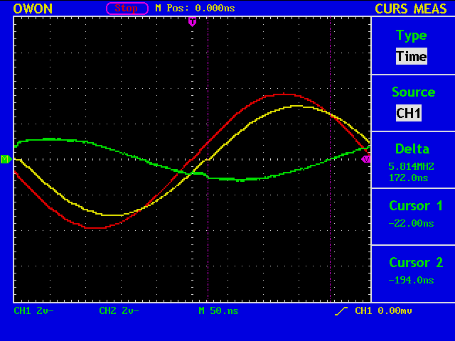
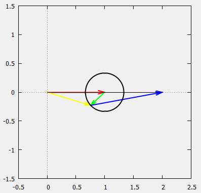
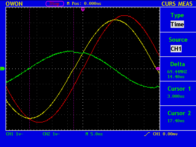
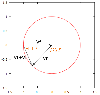
AT 7026kHz (T=142.3nS). The delay is -23.60nS (-59.7deg), V1=2.695V and V2=2.584V both measured using CH1 (V2/V1=0.959).

(%i) t:2.0*360.0*(9.0/(300.0*0.67/7.026));
(%o) 226.5098507462687
(%i) tt:2.0*3.1416*(t/360.0);
(%o) 3.953351928358209
(%i) Vf:1.0+%i*0.0;
(%o) 1.0
(%i) Vr:cos(tt)+%i*sin(tt);
(%o) -0.72549907008898*%i-0.68822314644309
(%i) abs(Vf+Vr);
(%o) 0.78965416931327
(%i) atan(imagpart(Vf+Vr)/realpart(Vf+Vr))/(2.0*3.1416)*360.0;
(%o) -66.74465370955055

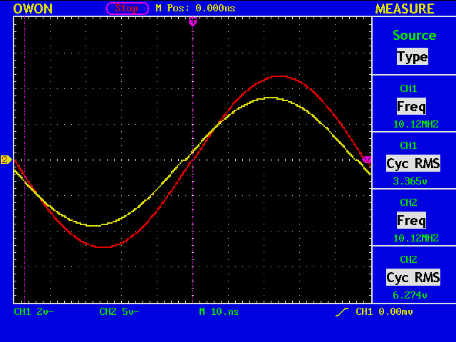
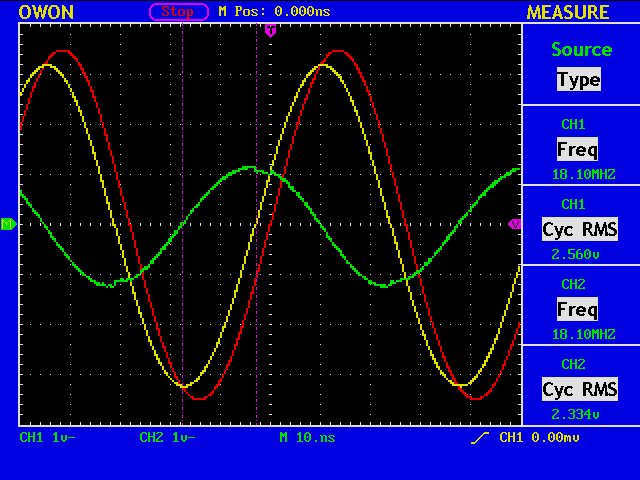
At 10120kHz (T=98.8nS). The delay is -2.40nS (-8.74deg)., V1=3.196V and V2=6.414V both measured using CH1 (V2/V1=2.01).

(%i) t:2.0*360.0*(9.0/(300.0*0.67/10.120));
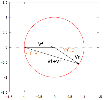
(%o) 326.2567164179104
(%i) tt:2.0*3.1416*(t/360.0);
(%o) 5.694267223880596
(%i) Vr:cos(tt)+%i*sin(tt);
(%o) 0.83154212893905-0.55546168886748*%i
(%i) Vf:1.0+%i*0.0;
(%o) 1.0
(%i) abs(Vf+Vr);
(%o) 1.913918560931499
(%i) atan(imagpart(Vf+Vr)/realpart(Vf+Vr))/(2.0*3.1416)*360.0;
(%o) -16.87122087372968

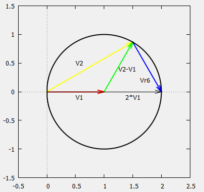
gnuplot> set size square
gnuplot> set xrange [-1.5:1.5]
gnuplot> set yrange [-1.5:1.5]
gnuplot> set zeroaxis
gnuplot> set parametric
gnuplot> x(t)=cos(t)
gnuplot> y(t)=sin(t)
gnuplot> plot [0:2*pi] x(t),y(t)
gnuplot> set arrow 1 from -1,0 to 0,0
gnuplot> set arrow 2 from  0,0 to 0.8794,0.4759
gnuplot> set arrow 3 from -1,0 to 0.4759,0.8794
gnuplot> replolt

GNU Radio is a free and open-source software development toolkit that provides signal processing blocks to implement software radios.

IC-7410 USB audio output is used as audio source.

Listening to a CW signal. CW pitch is set to 600Hz.

This is with a decimation filter.