もし、あなたがZ(DUT)だけでなく、あなたのアンテナの放射インピーダンスも知りたければ、あなたは、ケーブルの長さと短縮率に応じて、スミスチャート上で負荷の方向へ移動(反時計回りの回転)しなければなりません。
この図では、青色の点がZ(DUT)を、緑色のそれが放射インピーダンスを示しています。
freq1=7.02687 MHz, freq2=7.02978 MHz
amp(v2/v1)=0.778415, phase(v2/v1)=-0.53185 rad
v1=(1,0i), v2=(0.670893,-0.394757i), v3=(1.32911,0.394757i)
z=(0.382788,-0.410701i), z50=(19.1394,-20.535i)
gamma=(-0.329107,-0.394757i), abs=0.51395, arg=-129.818 deg
vswr=3.1148
cable_length=20 m, velocity_factor=0.67, phase_toward_load=143 deg
// file name = mytest46.cc
{
ifstream finput("owondata.txt");
Int_t iskip=8;
std::string s;
for(Int_t i=0;i<iskip;i++) {
getline(finput, s);
}
const Int_t icount_max=8192;
Int_t icount=0;
Double_t dummy, data1[icount_max], data2[icount_max], data3[icount_max];
while(icount < icount_max) {
finput >> data1[icount] >> dummy >> data2[icount] >> data3[icount];
if(finput.eof()) break;
icount++;
}
TCanvas *c1 = new TCanvas("c1","Test",0,0,800,600);
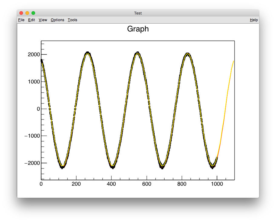
TGraph *g = new TGraph(icount, data1, data2);
g->SetMarkerStyle( 20 );
g->SetMarkerSize( 0.5 );
g->Draw("AP");
TF1 *f1 = new TF1("f1", "[0]*sin([1]*x+[2])-[3]");
f1->SetParameter(0, 2000.0);
f1->SetParameter(1, 0.022);
f1->SetParameter(2, 0.0);
f1->SetParameter(3, 0.0);
f1->SetLineColor(kRed);
g->Fit(f1);
TGraph *h = new TGraph(icount, data1, data3);
h->SetMarkerStyle( 24 );
h->SetMarkerSize( 0.5 );
h->Draw("P");
TF1 *f2 = new TF1("f2", "[0]*sin([1]*x+[2])-[3]");
f2->SetParameter(0, 2000.0);
f2->SetParameter(1, 0.022);
f2->SetParameter(2, 0.0);
f2->SetParameter(3, 0.0);
f2->SetLineColor(kYellow);
h->Fit(f2);
Double_t freq1, freq2;
const Double_t fsample = 2000.0; // MHz (interpolated)
freq1 = fsample / ( 2.0*TMath::Pi() / f1->GetParameter(1) );
freq2 = fsample / ( 2.0*TMath::Pi() / f2->GetParameter(1) );
std::cout << "freq1=" << freq1 << " MHz, freq2=" << freq2 << " MHz" << std::endl;
Double_t amp, phase;
amp = f2->GetParameter(0) / f1->GetParameter(0);
phase = f2->GetParameter(2) - f1->GetParameter(2);
std::cout << "amp(v2/v1)=" << amp << ", phase(v2/v1)=" << phase << " rad" << std::endl;
TComplex v1, v2, v3, Z, z50;
v1 = TComplex(1.0, 0.0);
v2 = TComplex( amp*TMath::Cos(phase), amp*TMath::Sin(phase) );
v3 = 2.0*v1 - v2;
z = v2/v3;
z50 = 50.0*z;
std::cout << "v1=" << v1 << ", v2=" << v2 << ", v3=" << v3 << std::endl;
std::cout << "z=" << z << ", z50=" << z50 << std::endl;
TComplex gg;
Double_t gg_rho, gg_theta, vswr;
gg = (z-1.0)/(z+1.0);
vswr = (1.0+TComplex::Abs(gg)) / (1.0-TComplex::Abs(gg));
std::cout << "gamma=" << gg
<< ", abs=" << gg.Rho()
<< ", arg=" << gg.Theta()*360.0/(2.0*TMath::Pi()) << " deg" << std::endl;
std::cout << "vswr=" << vswr << std::endl;
TCanvas * CPol = new TCanvas("CPol", "Test", 900, 0, 600, 600);
const Int_t ncircle = 360;
Double_t radius[ncircle];
Double_t theta [ncircle];
for (Int_t i=0; i<ncircle; i++) {
radius[i] = gg.Rho();
theta [i] = TMath::Pi()*2.0*(Double_t)i/(Double_t)(ncircle-1);
}
Double_t radius_r[ncircle];
Double_t theta_r [ncircle];
Double_t r_center = z.Re() / (z.Re()+1.0);
Double_t r_radius = 1.0 / (z.Re()+1.0);
for (Int_t i=0; i<ncircle; i++) {
Double_t th = TMath::Pi()*2.0*(Double_t)i/(Double_t)(ncircle-1);
Double_t re = r_center + r_radius*TMath::Cos(th);
Double_t im = r_radius*TMath::Sin(th);
TComplex ww = TComplex(re, im);
radius_r[i] = ww.Rho ();
theta_r [i] = ww.Theta();
}
Double_t radius_x[ncircle];
Double_t theta_x [ncircle];
TComplex x_center = TComplex(1.0, 1.0/z.Im());
Double_t x_radius = 1.0/ z.Im();
for (Int_t i=0; i<ncircle; i++) {
Double_t th = TMath::Pi()*2.0*(Double_t)i/(Double_t)(ncircle-1);
Double_t re = x_center.Re() + x_radius*TMath::Cos(th);
Double_t im = x_center.Im() + x_radius*TMath::Sin(th);
TComplex ww = TComplex(re, im);
radius_x[i] = ww.Rho ();
theta_x [i] = ww.Theta();
}
TGraphPolar * grP1 = new TGraphPolar(ncircle, theta, radius);
grP1->SetTitle("Smith Chart");
grP1->SetMarkerStyle(20);
grP1->SetMarkerSize(2.0);
grP1->SetMarkerColor(4);
grP1->SetLineColor(2);
grP1->SetLineWidth(3);
grP1->Draw("C");
CPol->Update();
grP1->GetPolargram()->SetToRadian();
grP1->GetPolargram()->SetRangeRadial(0,1);
TGraphPolar * grP2 = new TGraphPolar(ncircle, theta_r, radius_r);
grP2->SetMarkerStyle(20);
grP2->SetMarkerSize(2.0);
grP2->SetMarkerColor(4);
grP2->SetLineColor(9);
grP2->SetLineWidth(3);
grP2->Draw("C");
TGraphPolar * grP3 = new TGraphPolar(ncircle, theta_x, radius_x);
grP3->SetMarkerStyle(20);
grP3->SetMarkerSize(2.0);
grP3->SetMarkerColor(4);
grP3->SetLineColor(6);
grP3->SetLineWidth(3);
grP3->Draw("C");
TMarker *m0 = new TMarker(gg.Re(), gg.Im(), 20);
m0->SetMarkerSize(2.0);
m0->SetMarkerColor(4);
m0->Draw();
Double_t freq = (freq1+freq2)/2.0; // MHz
Double_t cable_length = 20.0; // meter
Double_t velocity_factor = 0.67;
Double_t wave_length = velocity_factor * (300.0 / freq);
Double_t phase_toward_load = 2.0 * 2.0 * TMath::Pi() * (cable_length / wave_length);
std::cout << "cable_length=" << cable_length
<< " m, velocity_factor=" << velocity_factor
<< ", phase_toward_load=" << (Int_t) ( phase_toward_load * 360.0 / (2.0*TMath::Pi()) ) % 360
<< " deg" << std::endl;
TComplex gg_toward_load = gg * TComplex::Exp(TComplex(0.0, phase_toward_load));
TMarker *m1 = new TMarker(gg_toward_load.Re(), gg_toward_load.Im(), 20);
m1->SetMarkerSize(2.0);
m1->SetMarkerColor(8);
m1->Draw();
}