今度は、周波数ミキサー、TAK-5です。

LO: 12.5MHz, RF: 5MHz.
LO: 12.5MHz, RF: 7.5Mhz.

LO: 15MHz, RF: 5MHz.

Ham Radio Blog
今度は、周波数ミキサー、TAK-5です。
LO: 12.5MHz, RF: 5MHz.
LO: 12.5MHz, RF: 7.5Mhz.
LO: 15MHz, RF: 5MHz.
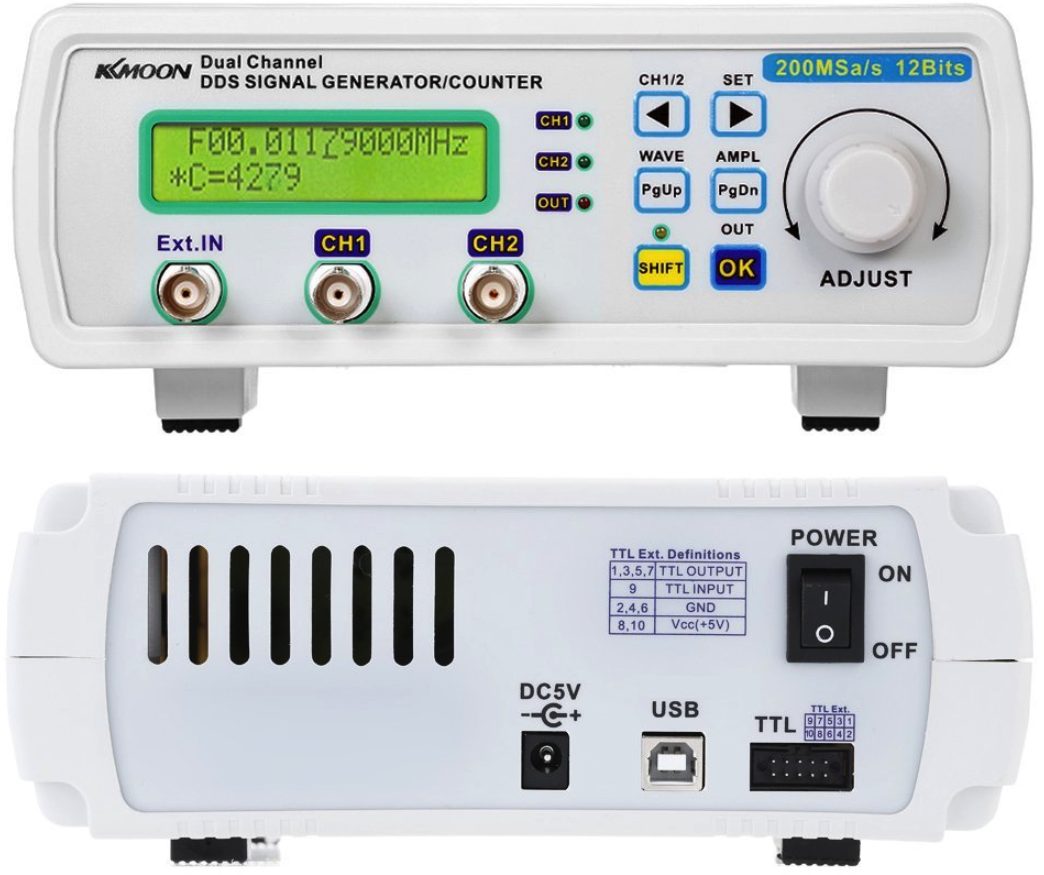
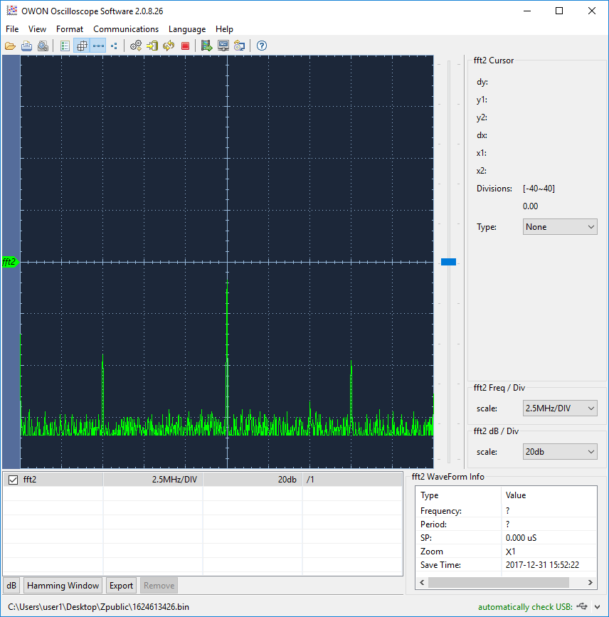
これは、私が最近入手した低価格の信号発生器です。

PSCQ-2-7.5という、パワー・スプリッター/コンバイナーで、少し実験をしてみましょう。
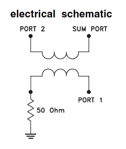
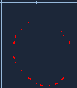
最初に、スプリッターとして:
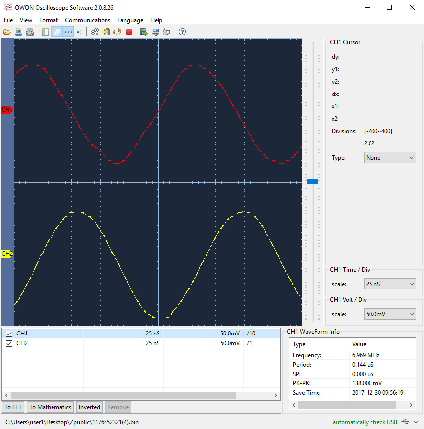
約7MHzの信号がsum portに加えられ、port 1とport 2からの信号が観測されます。2つの信号の位相差は90度のはずです。
次に、コンバイナーとして:
2つの信号、周波数が7010kHzと7110kHzですが、port Aとport Bとにそれぞれ加えられます。
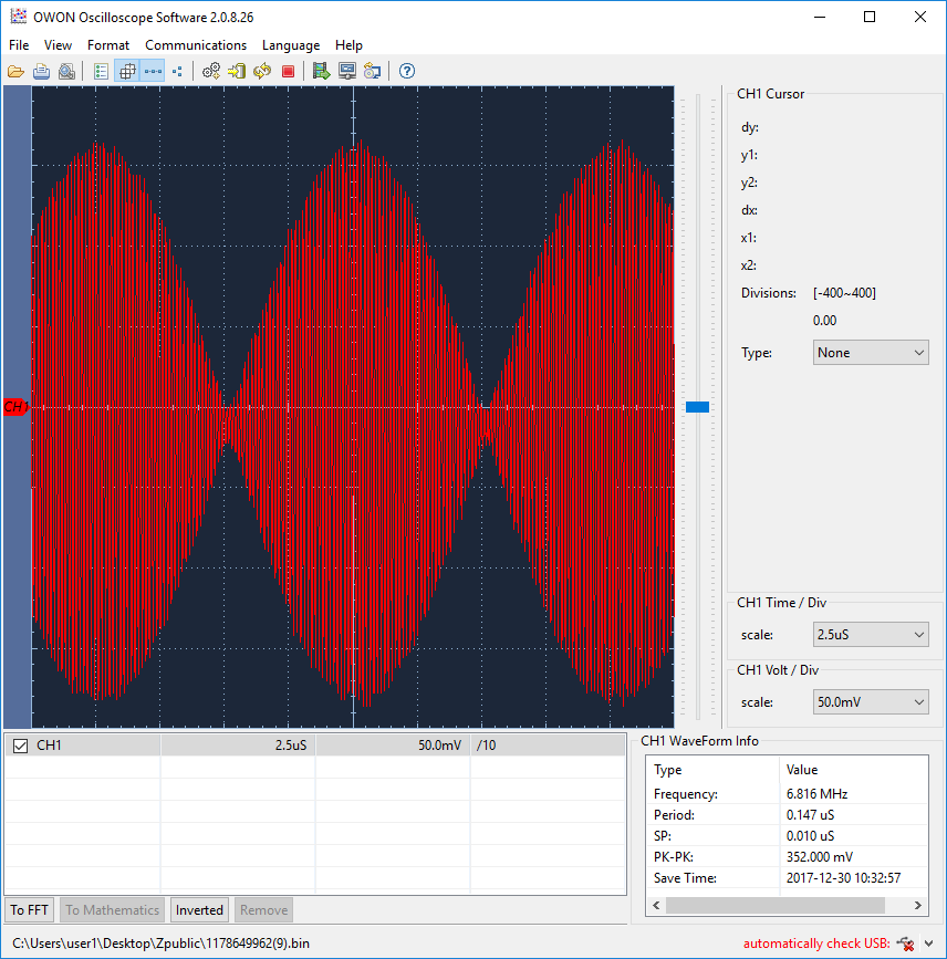
これが、sum portで観測されます。
私は20mの同軸ケーブル(5D-2V)を使っていますが、測定の最中はケーブルの遠端は開放にしておきます。
スミスチャートはあなたに全てを告げますが、それでも、振幅と位相とを別々に見た方が容易でしょう。
最初に、dBで表した振幅です。
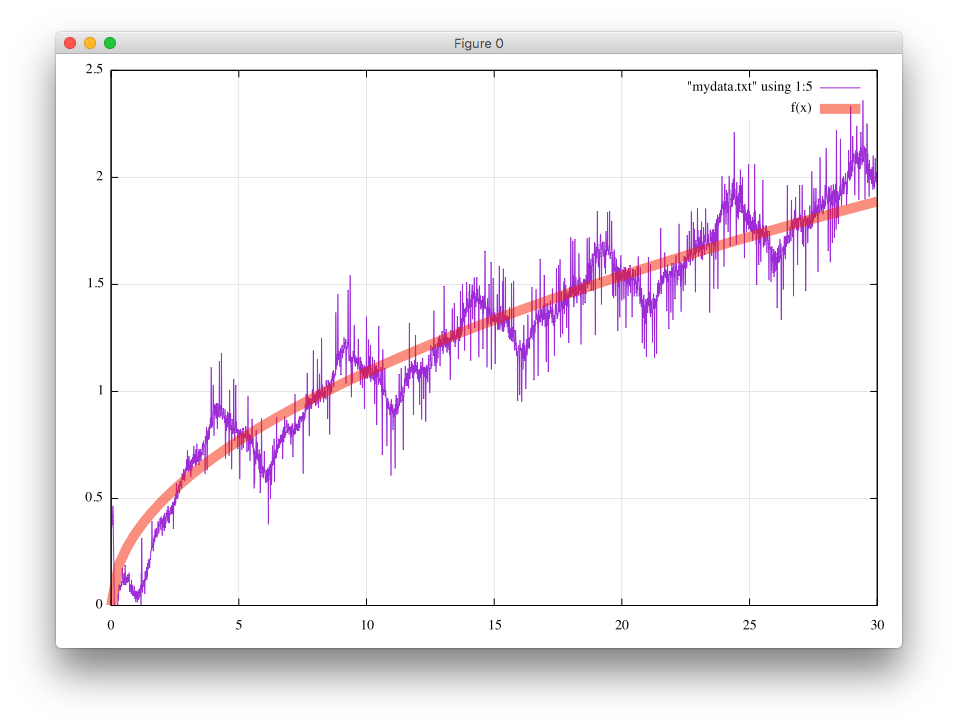
% gnuplot
gnuplot> f(x)=a*sqrt(x)
gnuplot> fit f(x) "mydata.txt" using 1:5 via a
iter      chisq       delta/lim  lambda   a
   0 9.0593050625e+02   0.00e+00  8.02e-01    2.070472e-01
   1 5.4539304323e+01  -1.56e+06  8.02e-02    3.445278e-01
   2 5.4539209850e+01  -1.73e-01  8.02e-03    3.445736e-01
iter      chisq       delta/lim  lambda   a

After 2 iterations the fit converged.
final sum of squares of residuals : 54.5392
rel. change during last iteration : -1.7322e-06

degrees of freedom    (FIT_NDF)                        : 3000
rms of residuals      (FIT_STDFIT) = sqrt(WSSR/ndf)    : 0.134832
variance of residuals (reduced chisquare) = WSSR/ndf   : 0.0181797

Final set of parameters            Asymptotic Standard Error
=======================            ==========================
a               = 0.344574         +/- 0.0006355    (0.1844%)
gnuplot> print a*sqrt(30)
1.88730727013936
30MHzでの損失1.887[dB]は、公称値の0.44dB/10m、すなわち、1.76dB/40mと良く一致します。
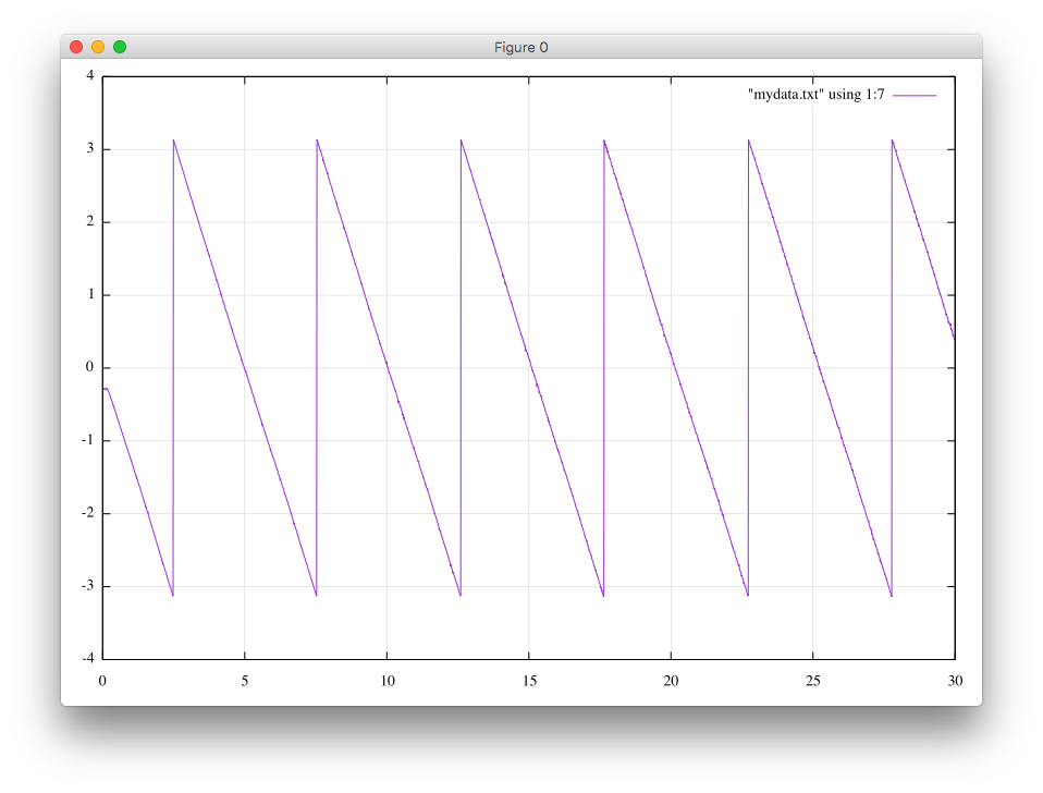
次に、ラジアンで表した位相です。
 .
.
位相がマイナスπから、プラスπに変化する周波数を見てみましょう。
 2.48, 1.3514, -0.299513, 1.3842, 0.469624, 36.9999, -3.1296, 0.947368
 2.49, 1.39451, 0.083306, 1.397, 0.484627, 35.8549, 3.13826, 0.945733

 7.53, 2.59869, -0.289392, 2.61476, 0.903662, 19.2411, -3.12999, 0.901191
 7.54, 2.45728, 0.08333, 2.4587, 0.854434, 20.3477, 3.13825, 0.906313

 12.6, 3.4673, -0.351551, 3.48508, 1.20654, 14.4212, -3.12746, 0.870308
 12.61, 3.43064, 0.097069, 3.43201, 1.1938, 14.5746, 3.13769, 0.871586
...
 27.77, 5.43172, -0.091826, 5.43249, 1.89464, 9.20522, -3.13788, 0.804022
 27.78, 5.31208, 0.100171, 5.31302, 1.85259, 9.41255, 3.13754, 0.807924
周期は (27.77MHz-2.48MHz)/5cyles、すなわち、5.06MHz/cycleです。
従ってケーブルの電気長は、(300m*MHz/5.06MHz)/2=29.64mです。
短縮率の66%を考慮すると、物理長は19.56mとなります。
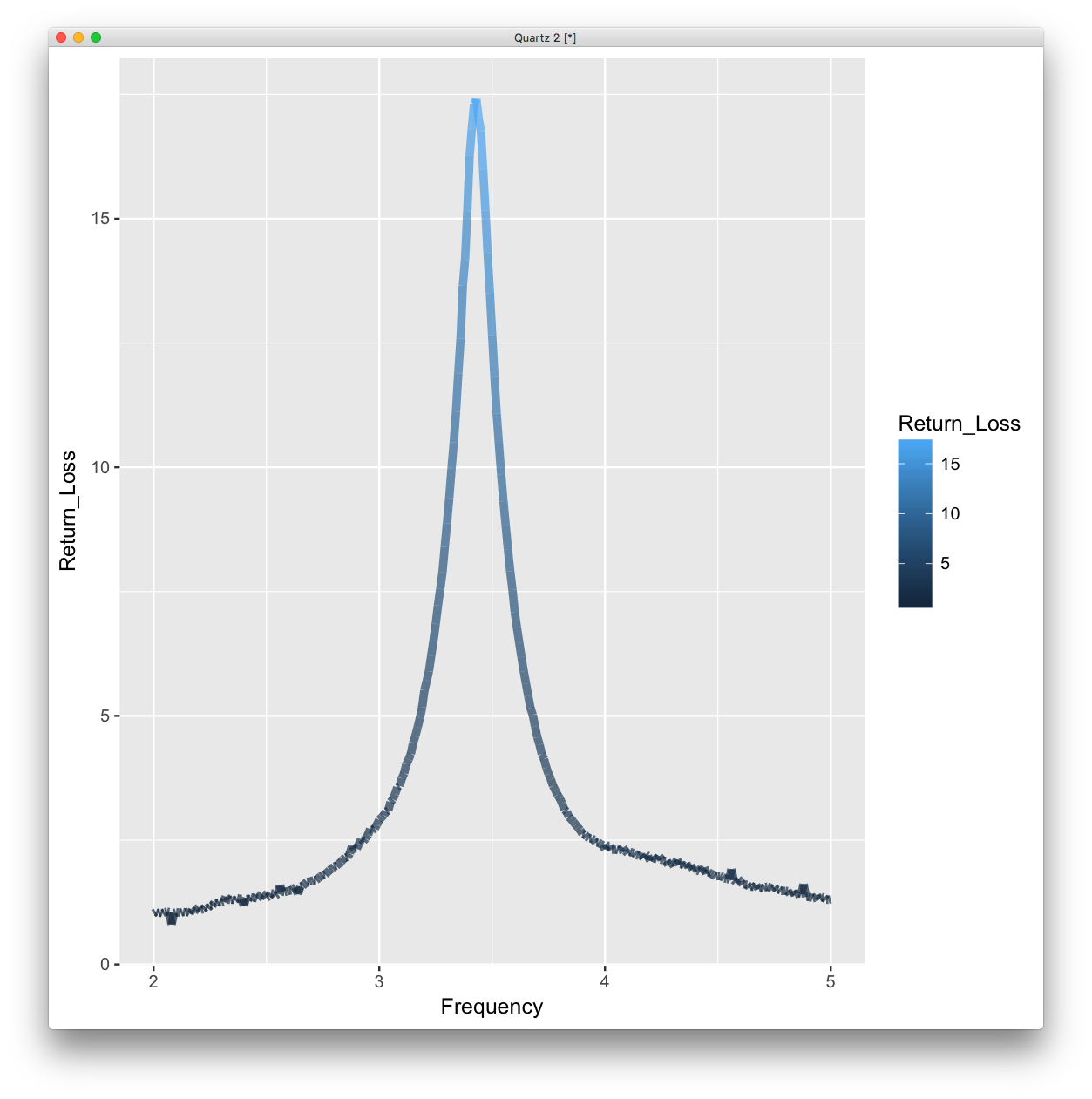
ggplot2を使うことは、Rでグラフを描くための別の方法です。
% head mydataR.txt
Frequency, R, X, Z, Return_Loss, VSWR, rhoAng, rhoAbs
2, 2.99567, -6.27359, 6.95212, 1.0258, 16.9545, -2.89108, 0.888607
2.01, 3.07187, -5.98362, 6.72608, 1.05344, 16.5107, -2.9025, 0.885784
2.02, 3.00247, -5.64513, 6.39393, 1.0312, 16.866, -2.91594, 0.888055
...
% R
> data<-read.table("mydataR.txt",sep=",",header=T)
> gp = ggplot(data, aes(x=Frequency, y=Return_Loss, colour=Return_Loss))
> gp = gp + geom_line(size=2, alpha=0.7)
> print(gp)
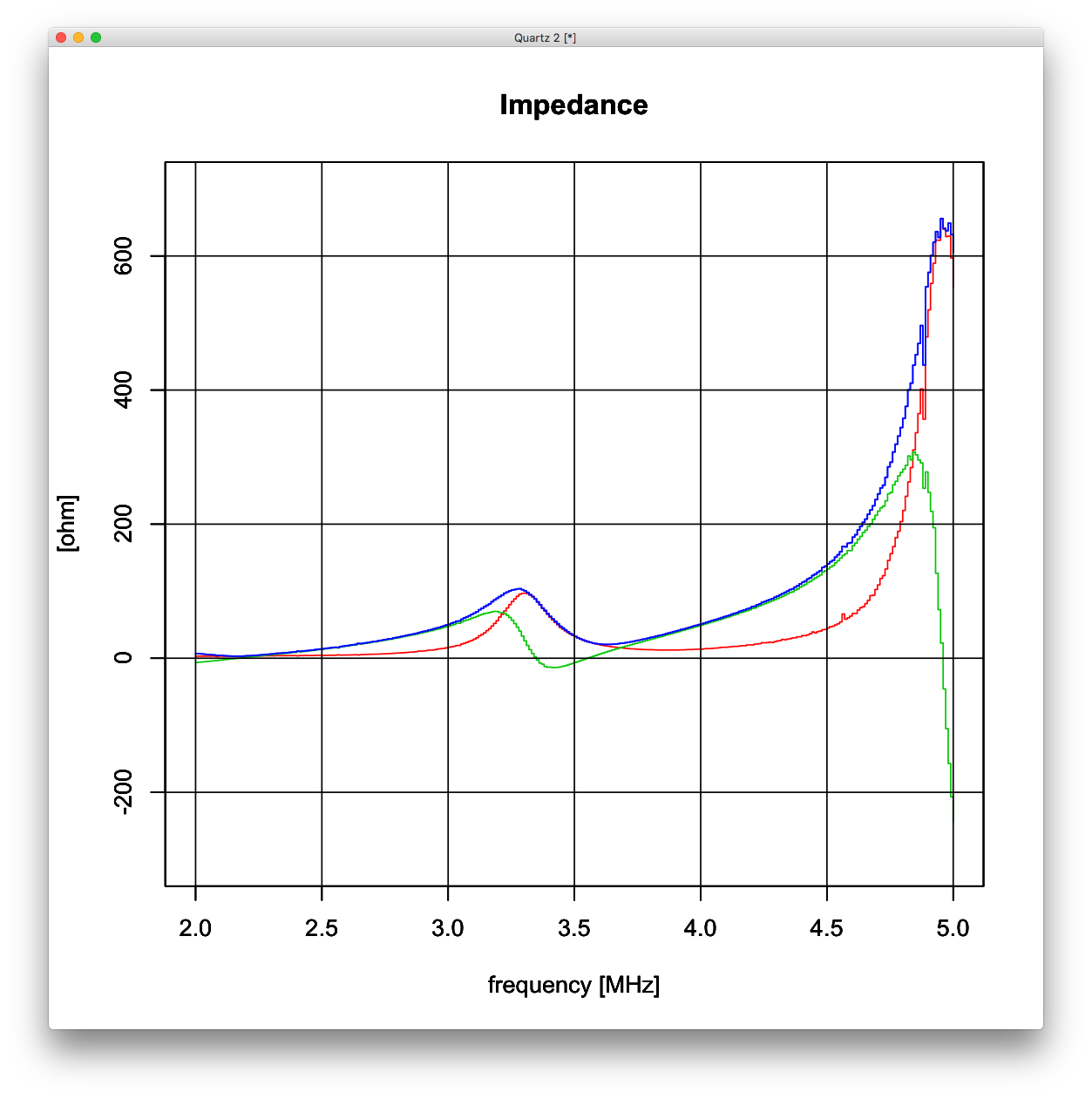
あなたは、またRをプロッティングに使うこともできます。
% R
> data<-read.table("mydata.txt",sep=",")
> plot(x=data$V1, y=data$V2, type="s", main="Impedance", xlab="frequency [MHz]", ylab="[ohm]", ylim=c(-300,700), col=2)
> par(new=T)
> plot(x=data$V1, y=data$V3, type="s", main="Impedance", xlab="frequency [MHz]", ylab="[ohm]", ylim=c(-300,700), col=3)
> par(new=T)
> plot(x=data$V1, y=data$V4, type="s", main="Impedance", xlab="frequency [MHz]", ylab="[ohm]", ylim=c(-300,700), col=4, tck=1)
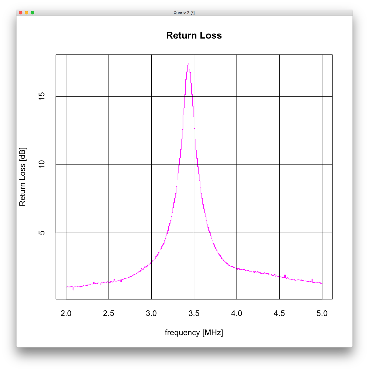
> plot(x=data$V1, y=data$V5, type="s", main="Return Loss", xlab="frequency [MHz]", ylab="Return Loss [dB]", col=6, tck=1)
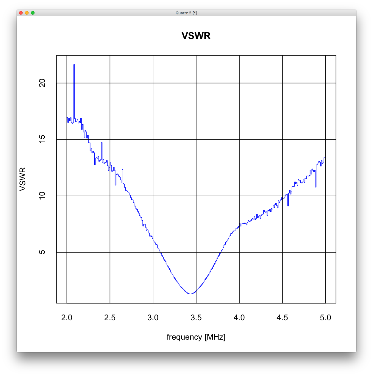
> plot(x=data$V1, y=data$V6, type="s", main="VSWR", xlab="frequency [MHz]", ylab="VSWR", col=4, tck=1)
もっと良い方法があるとは思いますが、これでも動きます。
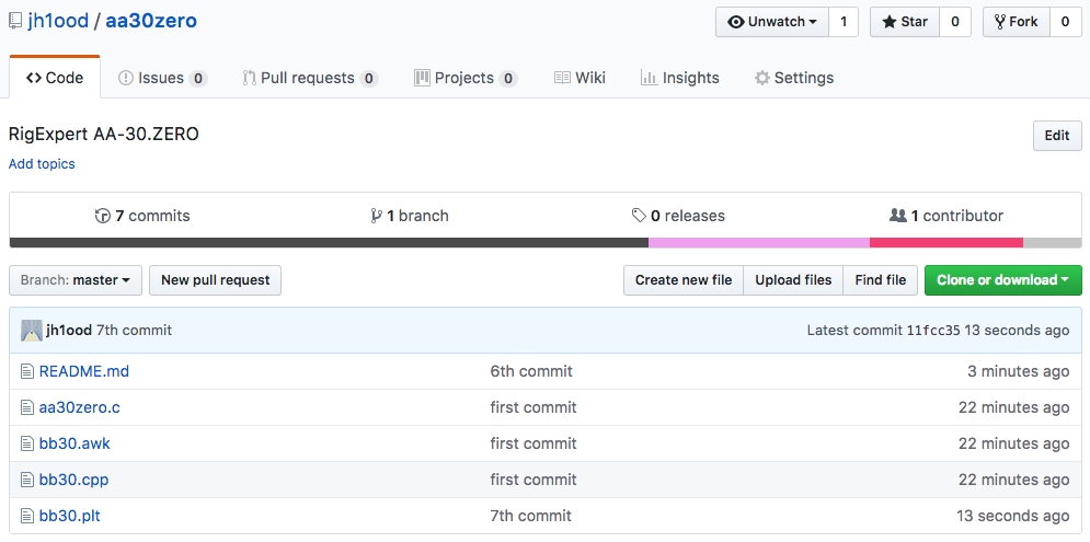
/* Data Converter for Rig Expert AA-30.ZERO */
/* % g++ bb30.cpp -o bb30 */
#include <complex>
#include <iostream>
#include <sstream>
#include <string>
using namespace std;

int main(int argc, char *argv[]) {
  string fval, rval, xval;
  double f, r, x;
  double absz, retloss, vswr;
  complex<double> z, rho;
  const complex<double> z0 = 50.0;

  while (!cin.eof()) {
    getline(cin, fval, ',');
    getline(cin, rval, ',');
    getline(cin, xval, '\n');

    stringstream(fval) >> f;
    stringstream(rval) >> r; if(r<0) r=0.01;
    stringstream(xval) >> x;

    z       = complex<double>(r,x);
    absz    = abs(z);
    rho     = (z-z0)/(z+z0);
    retloss = -20.0 * log( abs(rho) ) / log( 10.0 );
    vswr    = ( 1+abs(rho) ) / ( 1-abs(rho) );

    cout << f << ", " << r << ", " << x << ", " << absz << ", "
         << retloss << ", " << vswr << ", "
         << arg(rho) << ", " << abs(rho) << endl;
  }
}
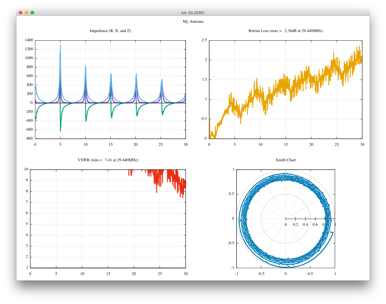
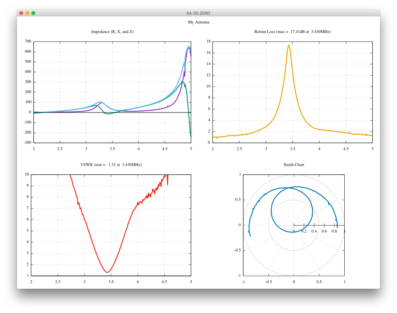
# Gnuplot script for AA-30.ZERO

reset
set terminal aqua enhanced title 'AA-30.ZERO' size 1200 900
set multiplot layout 2,2 title 'My Antenna'
set grid
unset key

fname = 'mydata.txt'
set datafile separator ','

set title 'Impedance (R, X, and Z)'
plot   fname using 1:2 with line linewidth 3, \
       ''    using 1:3 with line linewidth 3, \
       ''    using 1:4 with line linewidth 3, \
       0.0             with line linewidth 3 lc "#80000000"

stats '' using 1:5 nooutput
set title sprintf("Retrun Loss (max = %6.2fdB at %6.3fMHz)", STATS_max_y, STATS_pos_max_y)
plot '' using 1:5 with line linewidth 3 linetype 4


stats '' using 1:6 nooutput
set title sprintf("VSWR (min = %6.2f at %6.3fMHz)", STATS_min_y, STATS_pos_min_y)
set yrange [1:10]
plot '' using 1: 6 with line linewidth 3 linetype 7, \
     1.0           with line linewidth 3 lc "#80000000"

set title 'Smith Chart'
set polar
set grid polar
set size square
set xrange [-1:+1]
set yrange [-1:+1]
plot '' using 7:8 with line linewidth 3 linetype 6

unset multiplot
reset
% ./aa30zero /dev/cu.usbmodem1461 fq3500000 sw3000000 frx300 | ./bb30 > mydata.txt
この方が、読みやすいでしょうか。
# Gnuplot script for AA-30.ZERO

reset
set terminal aqua enhanced title 'AA-30.ZERO' size 1200 900
set multiplot layout 2,2 title 'My Antenna'
set grid
unset key

fname = 'mydata.txt'
set datafile separator ','

z0         = 50.0
z(r,x)     = r + x*{0,1}
rho(z)     = (z-z0)/(z+z0)
retloss(z) = -20.0 * log( abs(rho(z)) ) / log( 10.0 )
vswr(z)    = ( 1+abs(rho(z)) ) / ( 1-abs(rho(z)) )

set title 'Impedance (R, X, and Z)'
plot   fname using 1:( abs(z($2,$3)) ) with line linewidth 3, \
       ''    using 1:2                 with line linewidth 3, \
       ''    using 1:3                 with line linewidth 3, \
       0.0                             with line linewidth 3 lc "#80000000"

set title 'Return Loss'
plot '' using 1:( retloss(z($2,$3)) ) with line linewidth 3 linetype 4

set title 'VSWR'
plot '' using 1:( vswr   (z($2,$3)) ) with line linewidth 3 linetype 7, \
     1.0                              with line linewidth 3 lc "#80000000"

set title 'Smith Chart'
set polar
set grid polar
set size square
set xrange [-1:+1]
plot '' using ( arg(rho(z($2,$3))) ) : ( abs(rho(z($2,$3))) ) : (3*$1) with line linewidth 3 linetype 6

unset multiplot
reset
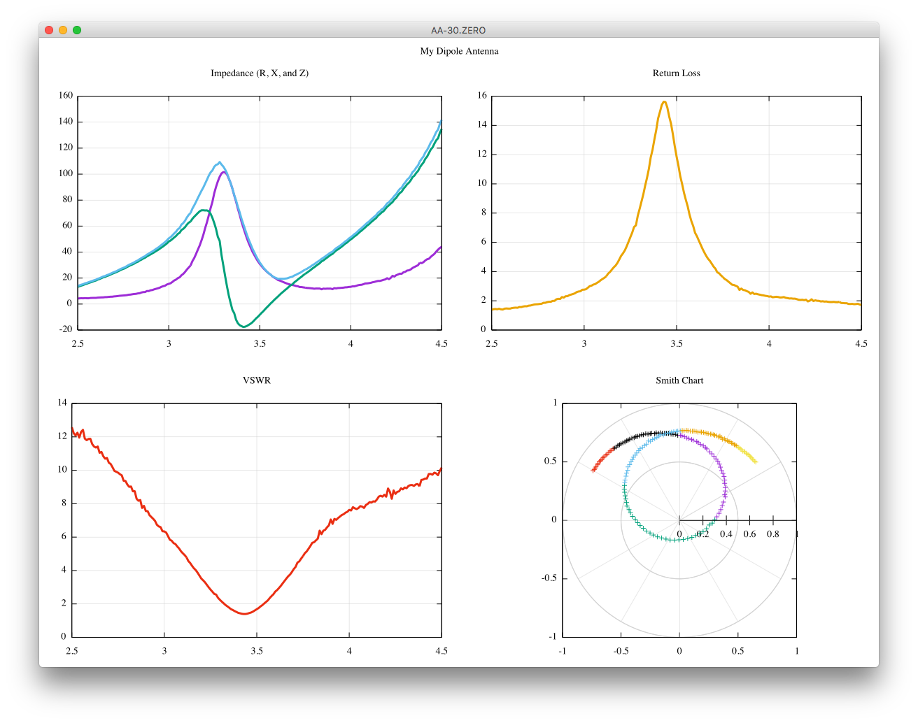
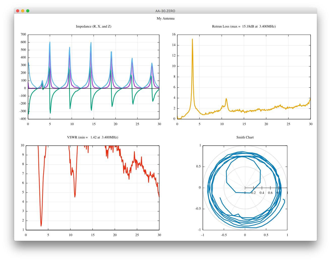
Gnuplotを用いれば、簡単に素敵なグラフを描くことができます。
あなたのAA-30.ZEROからの生データはこんな感じです:
...
2.990000,15.066906,46.652055
3.000000,15.557470,48.099209
3.010000,16.004803,48.884680
...
そして、スクリプトは:
# Gnuplot script for AA-30.ZERO
reset
set terminal aqua enhanced title "AA-30.ZERO" size 1200 900
set datafile separator ","
set grid
unset key
set multiplot layout 2,2 title "My Dipole Antenna"

set title "Impedance (R, X, and Z)"
plot   "mydata.txt" using 1:2 with line linewidth 3, \
"mydata.txt" using 1:3 with line linewidth 3, \
"mydata.txt" using 1:( abs($2+$3*{0,1}) ) with line linewidth 3

set title "Return Loss"
plot "mydata.txt" using 1:( -20.0 * log(abs( ($2+$3*{0,1}-50)/($2+$3*{0,1}+50) )) / log(10) ) with line linewidth 3 linetype 4

set title "VSWR"
plot "mydata.txt" using 1:( (1+abs( ($2+$3*{0,1}-50)/($2+$3*{0,1}+50) )) / (1-abs( ($2+$3*{0,1}-50)/($2+$3*{0,1}+50) )) ) with line linewidth 3 linetype 7

set title "Smith Chart"
set polar
set grid polar
set size square
set xrange [-1:+1]
plot "mydata.txt" using (arg( ($2+$3*{0,1}-50)/($2+$3*{0,1}+50) )) : (abs( ($2+$3*{0,1}-50)/($2+$3*{0,1}+50) )) : (3*$1) with point pointtype 7 lc variable

unset multiplot
ターミナルタイプはあなたのプラットフォームに応じて設定して下さい。スクリプトの3行目を見て下さい。
そして、あなたがすることはこれだけです。
% ./aa30zero fq3500000 sw2000000 frx200 > mydata.txt
% gnuplot aa30zero.plt