
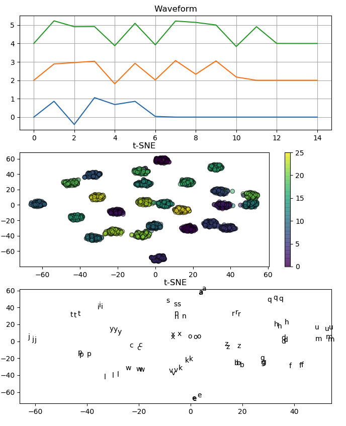
t-distributed Stochastic Neighbor Embedding (t-SNE)は、高次元のデータを可視化するためのツールです。
モールスコードでaからzを表している波形を、t-SNEを用いて2次元で可視化しています。
各信号は電気的に生成された後、ガウス雑音が加えられています。
import matplotlib.pyplot as plt
import numpy as np
from sklearn.manifold import TSNE

alphabet = list("abcdefghijklmnopqrstuvwxyz")

values = ['101110', '1110101010', '111010111010', '11101010', '10',
          '1010111010', '1110111010', '10101010', '1010', '10111011101110',
          '1110101110', '1011101010', '11101110', '111010', '111011101110',
          '101110111010', '11101110101110', '10111010', '101010', '1110',
          '10101110', '1010101110', '1011101110', '111010101110', '11101011101110',
          '111011101010']

morse_dict = dict(zip(alphabet, values))

nrepeat = 100
n = len(values)
word_len = 15

X = np.zeros((n * nrepeat, word_len))
Y = np.zeros(n * nrepeat, dtype=np.int)

for rep in range(nrepeat):
    for i, letter in enumerate(alphabet):
        for j, char in enumerate(morse_dict[letter]):
            X[i+rep * n][j+1] = (ord(char) - ord('0')) + np.random.normal(0.0, 0.2)
            Y[i+rep * n] = i

X_reduced = TSNE(n_components=2, random_state=0).fit_transform(X)

plt.figure(figsize=(8, 12))

plt.subplot(3, 1, 1)
x = np.arange(word_len)
for i in range(3):
    y = X[i, :] + 2.0 * i
    plt.plot(x, y)
plt.grid()
plt.title('Waveform')

plt.subplot(3, 1, 2)
plt.scatter(X_reduced[:, 0], X_reduced[:, 1],
            c=Y, edgecolors='black', alpha=0.5)
plt.colorbar()
plt.title('t-SNE')

plt.subplot(3, 1, 3)
for rep in range(min(3, nrepeat)):
    for i, letter in enumerate(alphabet):
        s = chr(Y[i] + ord('a'))
        plt.text(X_reduced[i+rep*n, 0], X_reduced[i+rep*n, 1], s)
plt.xlim([min(X_reduced[:, 0]), max(X_reduced[:, 0])])
plt.ylim([min(X_reduced[:, 1]), max(X_reduced[:, 1])])
plt.title('t-SNE')

plt.show()