
![]()
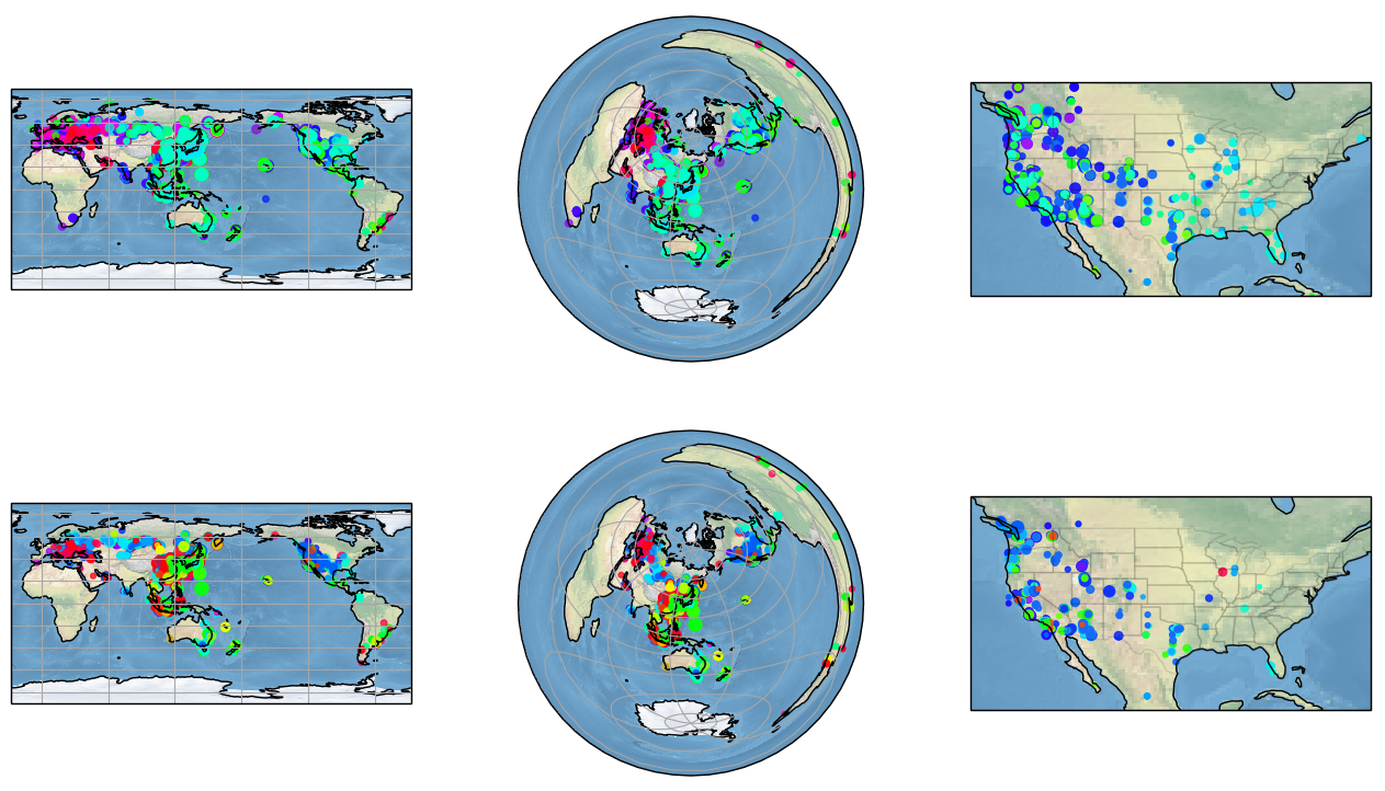
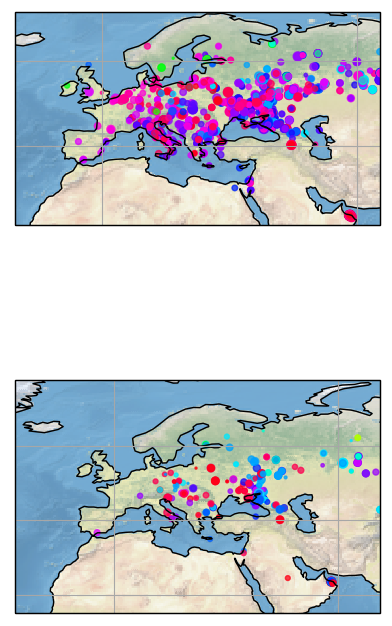
あなたは拡大鏡アイコンをクリックして、地図にズームインすることが出来ます。
import cartopy
import cartopy.crs as ccrs
import cartopy.feature as cfeature
import shapely.geometry as sgeom
import cartopy.io.shapereader as shpreader
import matplotlib.pyplot as plt
import numpy as np
import re
import datetime

def maiden2lonlat(maiden: str):
    n = len(maiden)
    maiden = maiden.lower()
    aaa = ord('a')
    lon = -180.0
    lat = -90.0

    lon += (ord(maiden[0])-aaa)*20.0
    lat += (ord(maiden[1])-aaa)*10.0
    lon += int(maiden[2])*2.0
    lat += int(maiden[3])*1.0
    if n >= 6:
        lon += (ord(maiden[4])-aaa) * 5.0/60.0
        lat += (ord(maiden[5])-aaa) * 2.5/60.0
    if n >= 8:
        lon += int(maiden[6]) * 5.0/600.0
        lat += int(maiden[7]) * 2.5/600.0
    return lon, lat

def parse_adif(fn):
    raw = re.split('<eor>|<eoh>',open(fn).read() )
    raw.pop(0)
    raw.pop()
    logbook =[]
    for record in raw:
        qso = {}
        tags = re.findall('<(.*?):\d+.*?>([^<\t\n\r\f\v]+)',record)
        for tag in tags:
            qso[tag[0]] = tag[1]
        logbook.append(qso)
    return logbook

def mydatetime(date, time):
    dt = datetime.datetime(int(date[0:4]), int(date[4:6]), int(date[6:8]), \
                           int(time[0:2]), int(time[2:4]), int(time[4:6]))
    return dt


fnames = ['station1.adif', 'station2.adif']

dt0 = datetime.datetime(2001,  1,  1,  0, 0 ,  0)
dt9 = datetime.datetime(2099, 12, 31, 23, 59, 59)

fig = plt.figure(figsize=(16, 9))

fcount = 0
for fn in fnames:
    x = []
    y = []
    r = []
    c = []
    log = parse_adif(fn)
    scount = 0
    for qso in log:
        if ('GRIDSQUARE' in qso):
            dt = mydatetime(qso['QSO_DATE'], qso['TIME_ON'])
            mytime = qso['TIME_ON']
            myhour = float(mytime[0:2])
            if dt >= dt0 and dt <=dt9:
                grid = qso['GRIDSQUARE']
                mylon, mylat = maiden2lonlat(grid)
                if ('APP_PSKREP_SNR' in qso):
                    snr = float(qso['APP_PSKREP_SNR'])
                    print(fcount, scount, grid, mylon, mylat, snr, mytime, myhour)
                    x.append(mylon)
                    y.append(mylat)
                    r.append(50.0+2.0*snr)
                    c.append(myhour/24.0)
                    scount += 1


    cent_lon = 152.5
    ax = fig.add_subplot(2, 3, 1+3*fcount, projection=ccrs.PlateCarree(central_longitude=cent_lon))
    ax.stock_img()
    ax.gridlines()
    ax.coastlines()
    ax.scatter(np.subtract(x,cent_lon), y, c=c, s=r, cmap='hsv', alpha=0.7)

    cent_lon = 139.7
    cent_lat = 35.7
    ax = fig.add_subplot(2, 3, 2+3*fcount, projection=ccrs.AzimuthalEquidistant(central_longitude=cent_lon, central_latitude=cent_lat))
    ax.stock_img()
    ax.gridlines()
    ax.coastlines()
    ax.scatter(x, y, c=c, s=r, cmap='hsv', alpha=0.7, transform=ccrs.Geodetic())

    ax = fig.add_subplot(2, 3, 3+3*fcount, projection=ccrs.PlateCarree())
    ax.stock_img()
    ax.coastlines()
    ax.set_extent([-130.0, -66.5, 20.0, 50.0], ccrs.Geodetic())
    shapename = 'admin_1_states_provinces_lakes_shp'
    states_shp = shpreader.natural_earth(resolution='110m', category='cultural', name=shapename)

    for state in shpreader.Reader(states_shp).geometries():
        facecolor = [0.9375, 0.9375, 0.859375]
        edgecolor = 'black'
        ax.add_geometries([state], ccrs.PlateCarree(),
                          facecolor=facecolor, edgecolor=edgecolor, alpha=0.1)

    ax.scatter(x, y, c=c, s=r, cmap='hsv', alpha=0.9)
    fcount += 1

plt.show()