リグエキスパートのAA-30.ZEROグラフ描画（４）

あなたは、またRをプロッティングに使うこともできます。

% R
> data<-read.table("mydata.txt",sep=",")
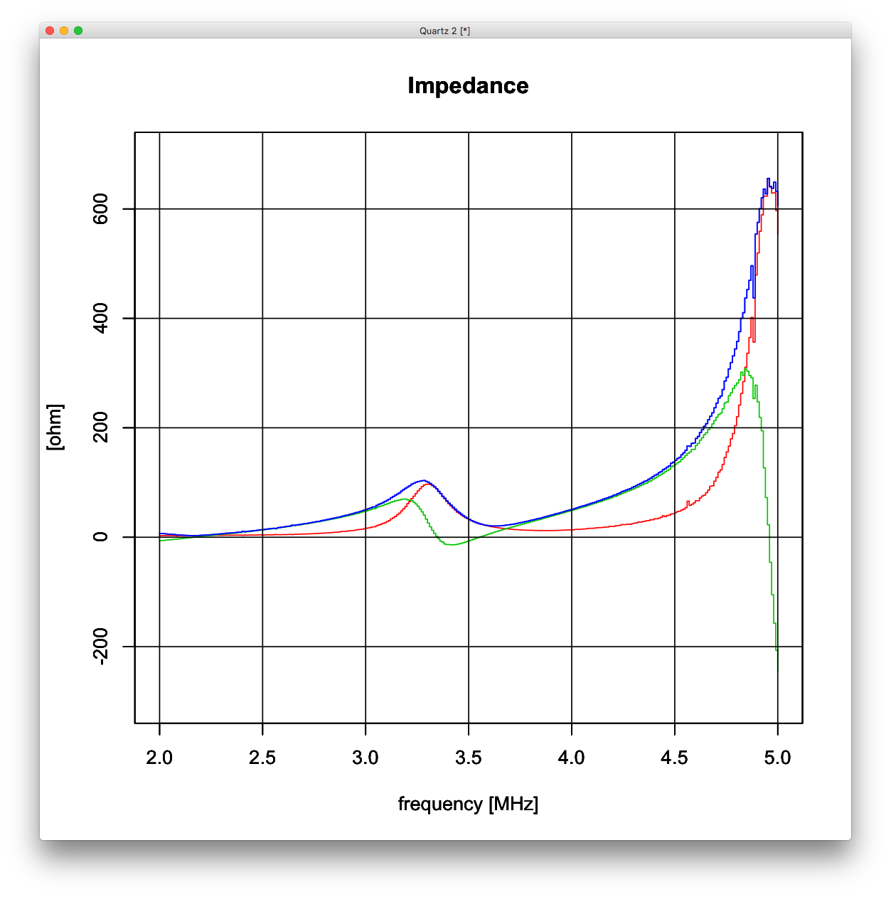
> plot(x=data$V1, y=data$V2, type="s", main="Impedance", xlab="frequency [MHz]", ylab="[ohm]", ylim=c(-300,700), col=2)
> par(new=T)
> plot(x=data$V1, y=data$V3, type="s", main="Impedance", xlab="frequency [MHz]", ylab="[ohm]", ylim=c(-300,700), col=3)
> par(new=T)
> plot(x=data$V1, y=data$V4, type="s", main="Impedance", xlab="frequency [MHz]", ylab="[ohm]", ylim=c(-300,700), col=4, tck=1)
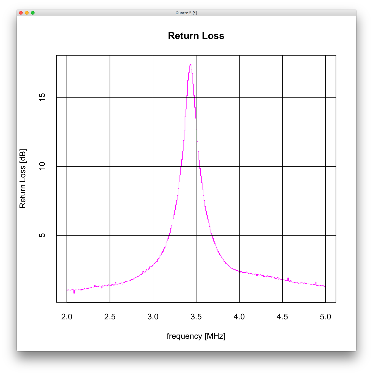
> plot(x=data$V1, y=data$V5, type="s", main="Return Loss", xlab="frequency [MHz]", ylab="Return Loss [dB]", col=6, tck=1)
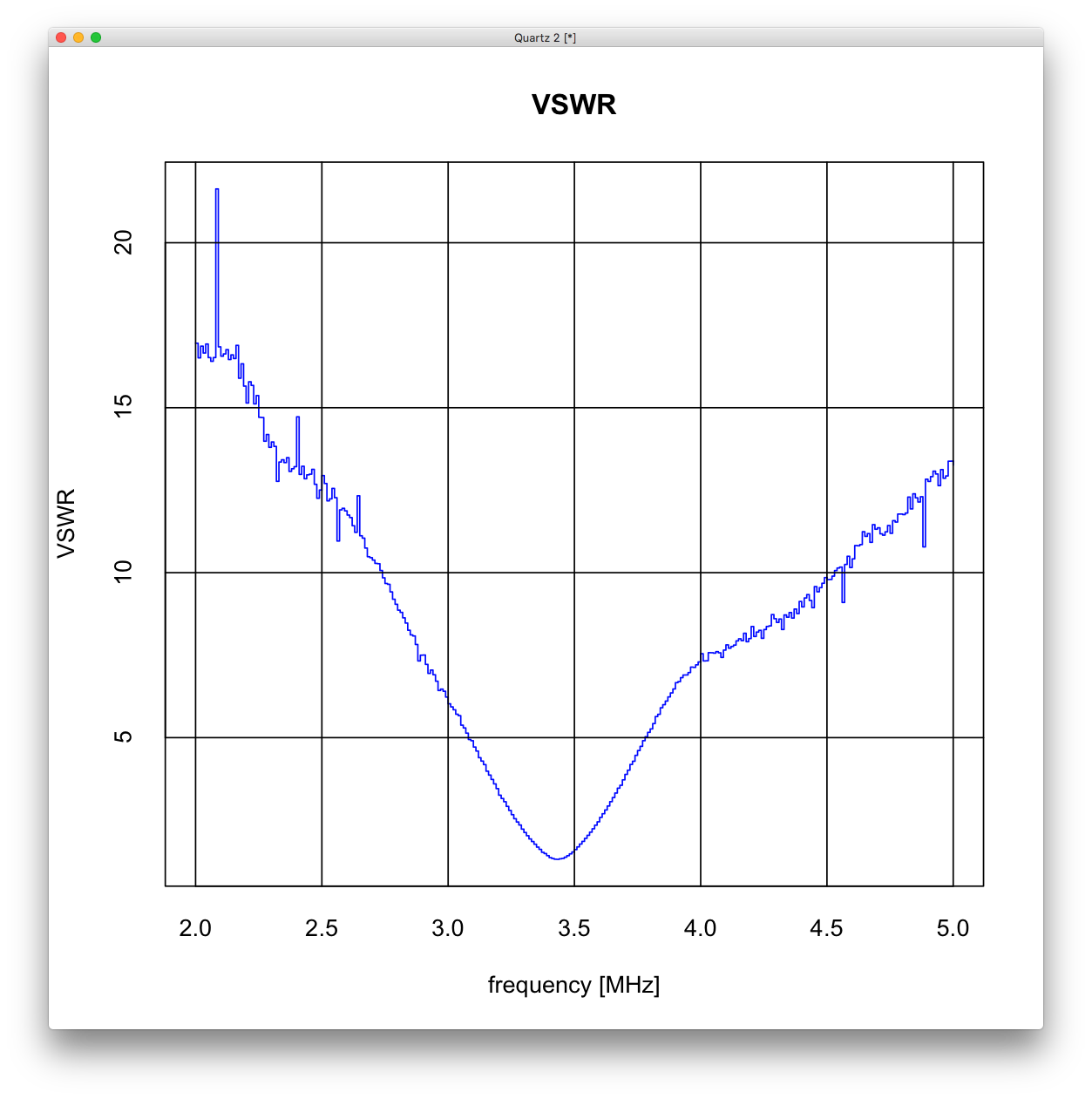
> plot(x=data$V1, y=data$V6, type="s", main="VSWR", xlab="frequency [MHz]", ylab="VSWR", col=4, tck=1)