さて、ATUで7038kHzに同調させた私のダイポールの測定をしてみましょう。
以下のような値が得られました。
...
7.037000 45.16 0.30
7.037500 45.31 0.19
7.038000 45.33 0.09
7.038500 45.29 -0.14
7.039000 45.28 -0.24
7.039500 45.44 -0.30
7.040000 45.31 -0.56
...
gnuplotを用いて、幾つかのグラフを描いてみます。
% gnuplot
gnuplot> plot "ant2.csv" using 1:2 with line linewidth 3,
          "ant2.csv" using 1:3 with line linewidth 3
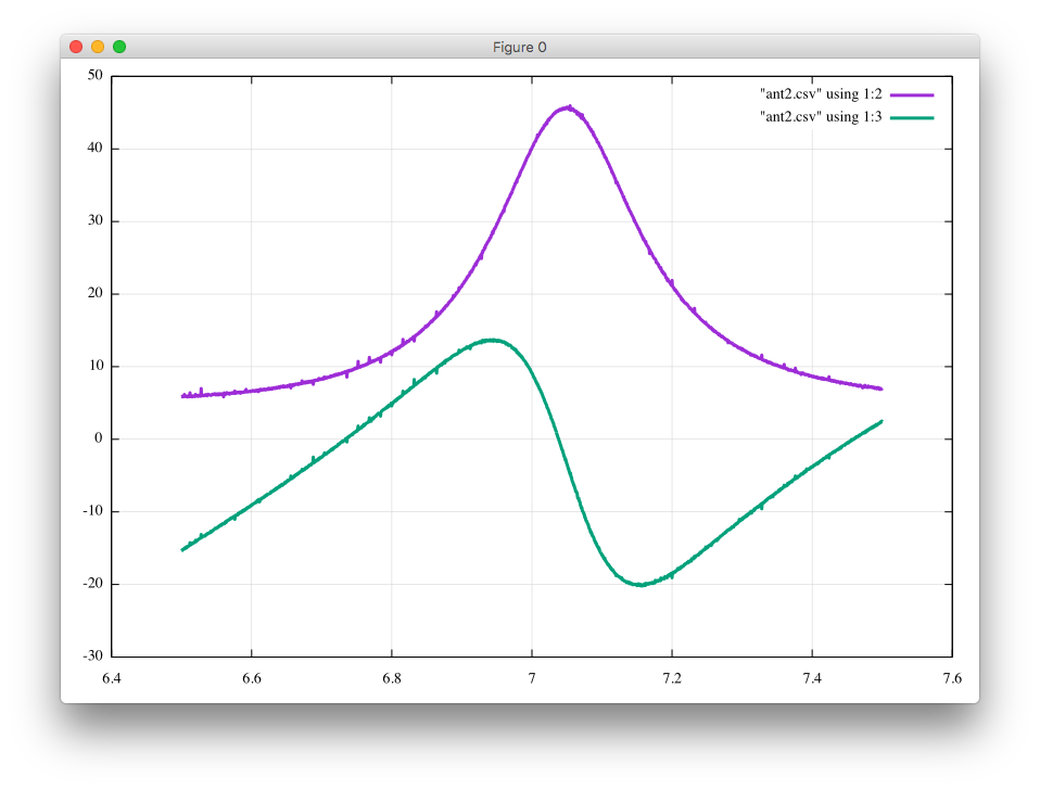
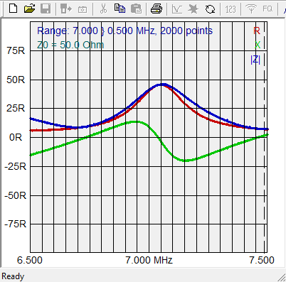
周波数範囲は、6.5MHzから7.5MHzで、紫色の線はR [ohm]、緑色の線はX [ohm]です。
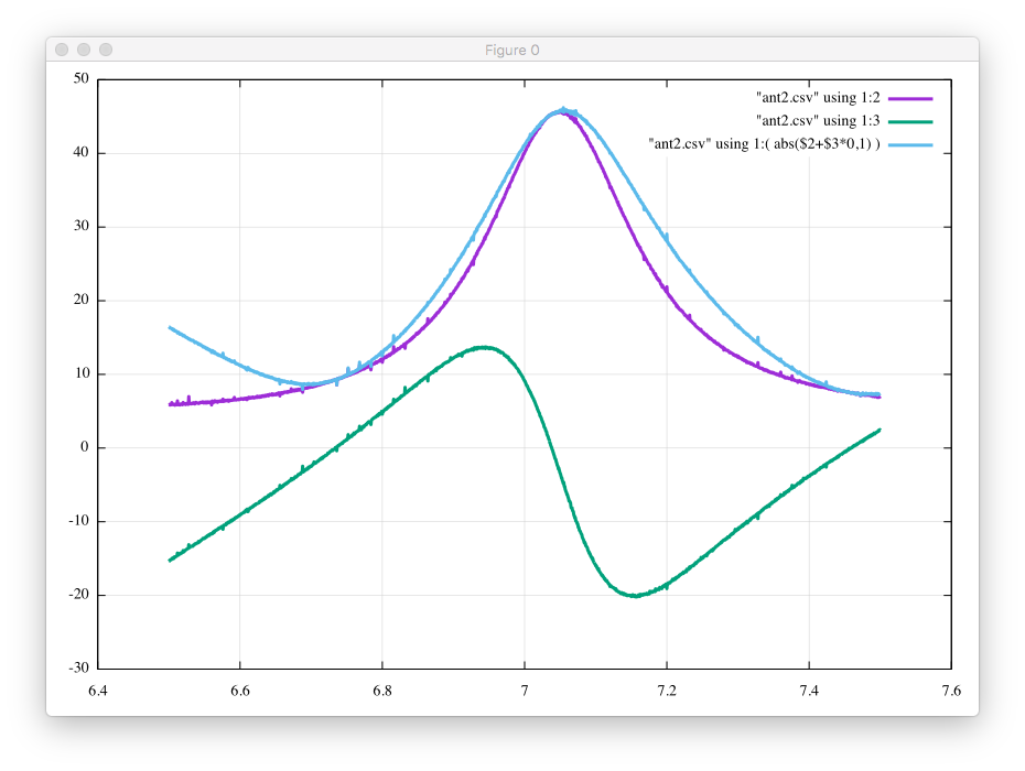
もし、|Z|も表示させたいのであれば、描画コマンドはこうなります。
gnuplot> plot "ant2.csv" using 1:2 with line linewidth 3, \
          "ant2.csv" using 1:3 with line linewidth 3, \
          "ant2.csv" using 1:( abs($2+$3*{0,1}) ) with line linewidth 3
AntScopeを用いれば同様のグラフを得ることはできますが、私はあなたが自分でそれをやりたいだろうと信じています。
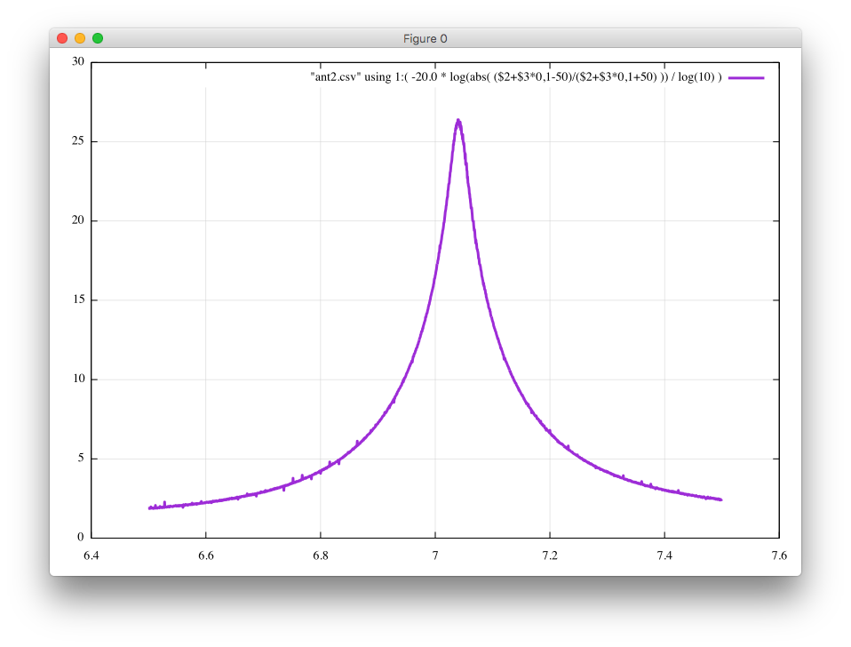
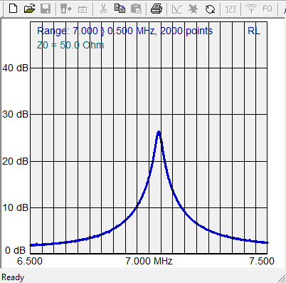
リターン・ロスは、以下のようにして求められます。
gnuplot> plot "ant2.csv" using 1:( -20.0 * log(abs( ($2+$3*{0,1}-50)/($2+$3*{0,1}+50) )) / log(10) ) with line linewidth 3
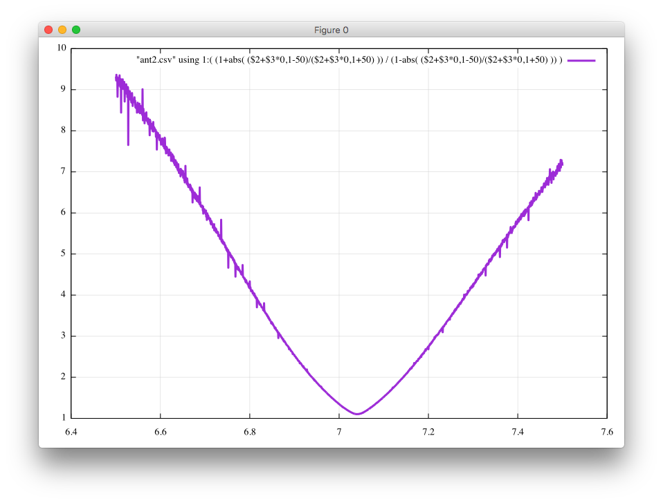
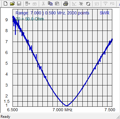
最後に、VSWRです。
gnuplot> plot "ant2.csv" using 1:( (1+abs( ($2+$3*{0,1}-50)/($2+$3*{0,1}+50) )) / (1-abs( ($2+$3*{0,1}-50)/($2+$3*{0,1}+50) )) ) with line linewidth 3