Antenna

The SWR meter tells you only the absolute value of the reflection coefficient. The impedance of your antenna is, in general, a complex number, and you can not determine both the real and the imaginary part of Zant from a single real number obtained from your SWR meter, such as SWR=1.2.

One method is to use an impedance bridge, which in this case is called a directional bridge.

Here is my implementation of a bridge. The RF signal comes from the left, goes through an attenuator, and your device under test (DUT) is on the right. The two probes for CH1 and CH2 are attached to the both sides of the “detector”, which is an open circuit.

(example 1)
The red and yellow traces are for CH1 and CH2, respectively. The green trace shows a CH2-CH1 signal. In this measurement, the DUT is an open circuit, so the CH2 signal is almost twice as large as the CH1 signal.

---

(example 2)
The DUT is a 50 ohm dummy load in this case. Since the bridge is almost perfectly balanced, the difference signal CH2-CH1 in green trace is nearly zero.

---

(example 3)
The DUT is a 100 ohm resistor. CH1/CH2 should be (50/(50+50))/(100/(50+100)=0.75, and the measured values are CH1=4.879 V and CH2=6.481 V, which results in CH1/CH2=0.753.

---

(example 4)
The DUT is a 1000 pF capacitor, which is 22.6 ohm at 7.026 MHz. Since Zdut=0.0-j22.6 ohm, you need to do your calculations with complex numbers, namely:
CH1/CH2=(50/(50+50))/((0.0-j22.6)/(50+(0.0-j22.6)))=0.5+j1.10=abs(1.21)+arg(65.6deg). Here arg(65.6deg) corresponds to the phase in advance of 25.9 nS (=1/7.026MHz*(65.6/360.0)).

The measured values are CH1/CH2=4.507/3.488=1.29, and CH1 is 25.0 nS in advance relative to CH2, both of which well agree with the above calculations.

It is convenient to have some scripts to calculate Zdut from the measured values of CH1 and CH2.

# gnuplot1.txt
set object 1 rectangle from screen 0,0 to screen 1,1 fillcolor rgb "#f0f0f0" behind
set size square
set xrange[-0.5:2.5]
set yrange[-1.5:1.5]
set zeroaxis
set parametric

# input data from measurement
freq=7.026e6
v1=4.507
v2=3.488
cursor1=-25.0e-9
cursor2=+0.0e-9

vratio=v2/v1
period=1/freq
phase1=2.0*pi*(cursor1/period)
phase2=2.0*pi*(cursor2/period)
phasedeg1=360*(cursor1/period)
phasedeg2=360*(cursor2/period)

I={0,1}
z0=50.0
cv1=1+I*0;
cv2=vratio*(cos(phase1)+I*sin(phase1))
cvfwd=cv1
cvrfl=cv2-cv1
cvr=2*cv1-cv2
cz=z0*(cv2/cvr)
gamma=cvrfl/cvfwd
swr=(1+abs(gamma))/(1-abs(gamma))

print "Freq [MHz]=", freq/1e6
print "V1=", v1
print "V2=", v2
print "Cursor 1=", cursor1
print "Cursor 2=", cursor2
print ""
print "vratio=", vratio
print "phase1 [deg]=", phasedeg1
print "phase2 [deg]=", phasedeg2
print ""
print "abs(gamma)=", abs(gamma)
print "swr=", swr
print "cz=", cz

set arrow 1 from 0,0 to 1,0 lw 2 lt 1
set arrow 2 from 0,0 to 2,0 lw 1 lt -1
set arrow 3 from 0,0 to real(cv2),imag(cv2) lw 2 lt 6
set arrow 4 from 1,0 to real(cv2),imag(cv2) lw 2 lt 2
set arrow 5 from real(cv2),imag(cv2) to 2,0 lw 2 lt 3
plot [0:2*pi] 1+abs(gamma)*cos(t),abs(gamma)*sin(t) lw 1 lt -1 notitle

pause -1

If we use (example 4) again, we obtain

gnuplot> load "gnuplot1.txt"
Freq [MHz]=7.026
V1=4.507
V2=3.488
Cursor 1=-2.5e-08
Cursor 2=0.0

vratio=0.773907255380519
phase1 [deg]=-63.234
phase2 [deg]=0.0

abs(gamma)=0.949672362078565
swr=38.7395960271799
cz={1.53085540665043, -21.5608049709462}

Note that the capacitor used in (example 4) should show Z=0.0-j22.6 ohm at 7.026 MHz if its nominal value of 1000 pF is correct.

This vector diagram is generated by the above gnuplot script. The red, yellow and green vectors correspond to CH1, CH2, and CH2-CH1 signals, respectively.

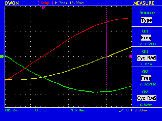
(example 5)
The DUT is a 5D-2V coax cable length 20 m with its end open circuited. The measured values of CH1=3.814 V, CH2=2.454 V, and CH2-delay=+25.0 nS give Zdut=2.5428-j17.6494 ohm.

The Smith Chart shows Zant=921.160+j412.077 ohm, very close to Zant=infinity.

---

(example 6)
The DUT is the same cable, but its end short circuited. The measured values of CH1=4.087 V, CH2=7.753 V, and CH2-delay=-6.2 nS give Zdut=9.244+j174.964 ohm.

The Smith Chart shows Zant=0.698+j2.106 ohm, very close to Zant=zero.

---

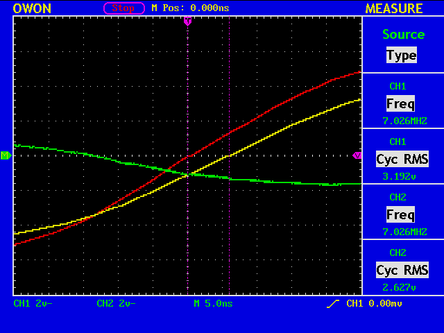
(example 7)
The DUT is the same cable, but is terminated with a 100 ohm resistor. The measured values of CH1=3.192 V, CH2=2.627 V, and CH2-delay=+6.0 nS give Zdut=9.244+j174.964 ohm.

The Smith Chart shows Zant=90.864+j9.986 ohm, close to the nominal value of 100 ohm.

---

(example 8)
The DUT is the same cable, but is terminated with a 1000 pF capacitor. The measured values of CH1=3.266 V, CH2=4.463 V, and CH2-delay=-14.8 nS give Zdut=9.914+j54.394 ohm.

The Smith Chart shows Zant=5.359-j21.793 ohm, close to the nominal value of 0.0-j22.6 ohm.

(example 9)
The DUT is my dipole antenna with a 20m 5D-2V coax cable. The dipole is not resonant at 40m band, because the whole length of the antenna is about 12.5 m. The measured values of CH1=2.093 V, CH2=892.2 mV, and CH2-delay=+25.0 nS give Zdut=2.961-j11.148 ohm.

Considering the cable length of 20 m, Zant=215.987-j378.040 ohm.

Since my dipole antenna in example 9 has Zant=215.987-j378.040 ohm, which is far from 50 ohm, we need some means to match the impedance. Here we use a stub match.

The first step is move to the point on the g=1 circle, and this step determines the “d1” in the above figure to be 5648.0 mm.

Note: The Zdut, Zant plus a 20m coax cable, in example 9 is on the g=1 circle, but this is only a coincidence. Naturally, 20 m – 5648.0 mm = 14.352 mm is half the wavelength at 7.026MHz considering the velocity factor.

The second step is to cancel the imaginary part with a stub. In this case, “d2” should be 1097.7 mm with its end short circuited. Then what you finally obtain is Z=48.855+j2.558 ohm. (Never mind the minor difference from Z=50.0+j0.0 ohm.) Now you can use a coax cable of any length between the transmitter and the stub.

You can easily obtain the solution for your stub matching at http://www.amanogawa.com/archive/SingleStub/SingleStub-2.html

It tells you that Dstub=0.19702 lambda=8.40665 m and Lstub=0.03924 lambda=1.674495 m, which translates to d1=5632.4 mm and d2=1121.9 mm considering the velocity factor of 0.67.

You can also use 75 ohm coax cables for your stub matching. In that case, d1=5448.9 mm and d2=1140.3 mm, which I am going to implement.

Here is my dipole antenna with a Stub Match and a 20 m 5D-2V coax cable. The measured values of CH1=2.538 V, CH2=2.820 V, and CH2-delay=+6.8 nS give Zdut=44.913-j33.225 ohm and SWR=2.00, which is well within a range an internal tuner of the rig works fine.

Considering the cable length of 20 m, Zant=54.290+j36.705 ohm. (The part of the reason for not attaining the perfect match is that I used a 5C-FV cable. The velocity factor of the cable is around 78%, which significantly differs from 67% of 5C-2V cables.)

At 7.150MHz, almost perfect match is attained. Compare the figure with that of the example 2 above, in which case a 50 ohm dummy load is used.