PythonとSciPy（２）

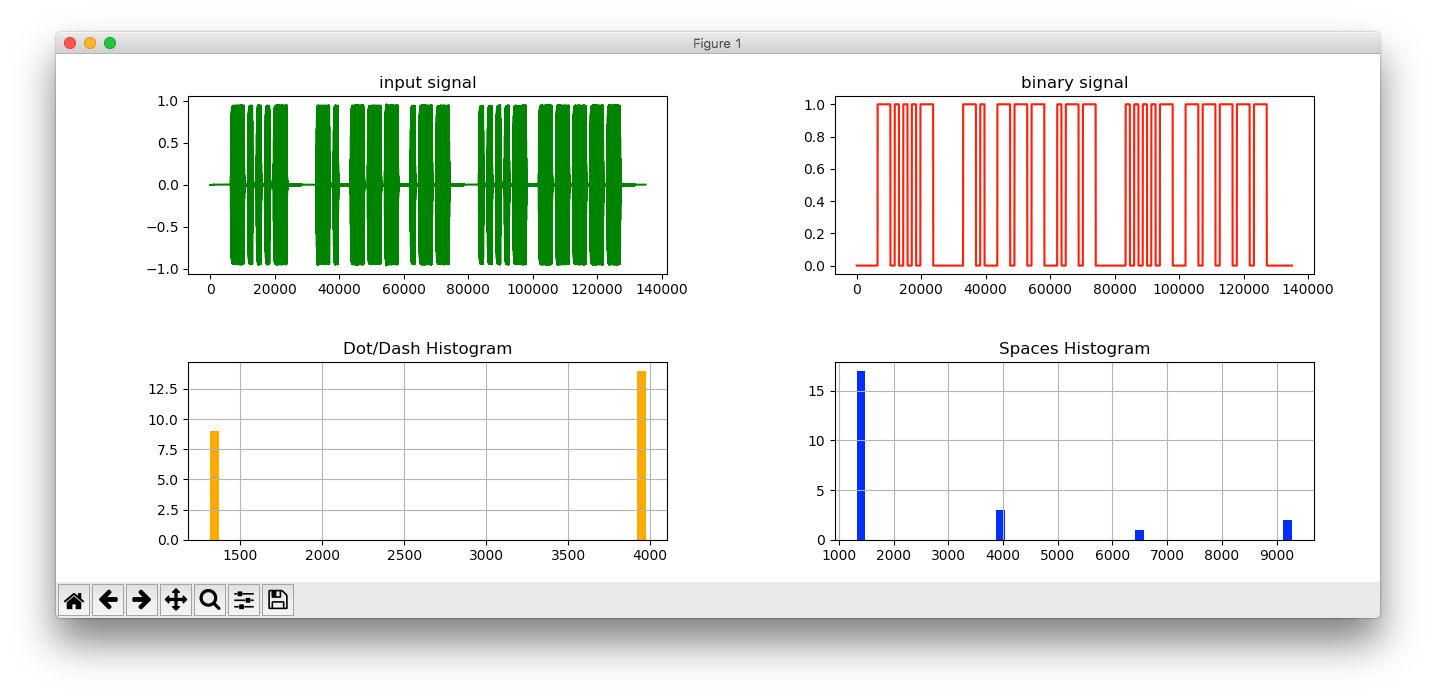
包絡線さえ得てしまえば、短点/長点の継続時間のヒストグラムを描くことは容易です。

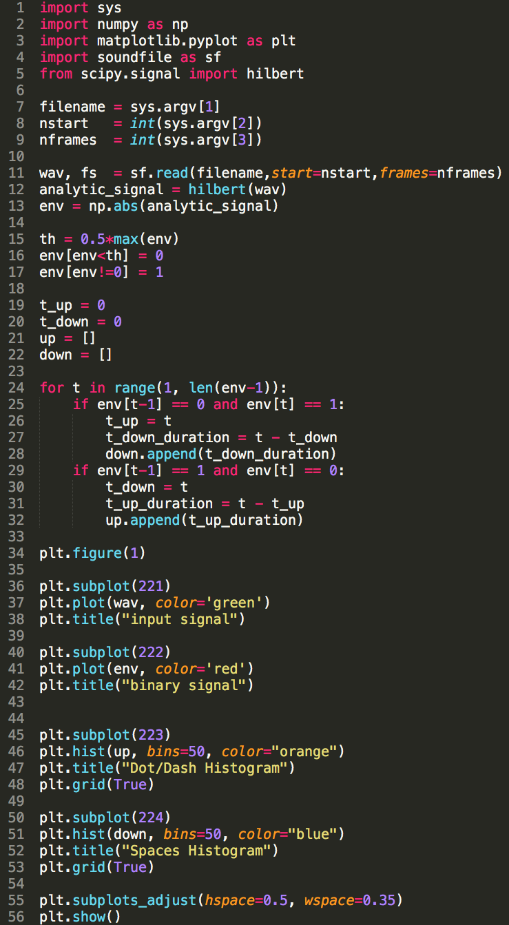
import sys
import numpy as np
import matplotlib.pyplot as plt
import soundfile as sf
from scipy.signal import hilbert

filename = sys.argv[1]
nstart   = int(sys.argv[2])
nframes  = int(sys.argv[3])

wav, fs  = sf.read(filename,start=nstart,frames=nframes)
analytic_signal = hilbert(wav)
env = np.abs(analytic_signal)

th = 0.5*max(env)
env[env<th] = 0
env[env!=0] = 1

t_up = 0
t_down = 0
up = []
down = []

for t in range(1, len(env-1)):
	if env[t-1] == 0 and env[t] == 1:
		t_up = t
		t_down_duration = t - t_down
		down.append(t_down_duration)
	if env[t-1] == 1 and env[t] == 0:
		t_down = t
		t_up_duration = t - t_up
		up.append(t_up_duration)

plt.figure(1)

plt.subplot(221)
plt.plot(wav, color='green')
plt.title("input signal")

plt.subplot(222)
plt.plot(env, color='red')
plt.title("binary signal")


plt.subplot(223)
plt.hist(up, bins=50, color="orange")
plt.title("Dot/Dash Histogram")
plt.grid(True)

plt.subplot(224)
plt.hist(down, bins=50, color="blue")
plt.title("Spaces Histogram")
plt.grid(True)

plt.subplots_adjust(hspace=0.5, wspace=0.35)
plt.show()